Co-Training Realized Volatility Prediction Model with Neural Distributional Transformation
DOI: https://doi.org/10.1145/3604237.3626870
ICAIF '23: 4th ACM International Conference on AI in Finance, Brooklyn, NY, USA, November 2023
This paper shows a novel machine learning model for realized volatility (RV) prediction using a normalizing flow, an invertible neural network. Since RV is known to be skewed and have a fat tail, previous methods transform RV into values that follow a latent distribution with an explicit shape and then apply a prediction model. However, knowing that shape is non-trivial, and the transformation result influences the prediction model. This paper proposes to jointly train the transformation and the prediction model. The training process follows a maximum-likelihood objective function that is derived from the assumption that the prediction residuals on the transformed RV time series are homogeneously Gaussian. The objective function is further approximated using an expectation–maximum algorithm. On a dataset of 100 stocks, our method significantly outperforms other methods using analytical or naïve neural-network transformations.
ACM Reference Format:
Xin Du, Kai Moriyama, and Kumiko Tanaka-Ishii. 2023. Co-Training Realized Volatility Prediction Model with Neural Distributional Transformation. In 4th ACM International Conference on AI in Finance (ICAIF '23), November 27--29, 2023, Brooklyn, NY, USA. ACM, New York, NY, USA 9 Pages. https://doi.org/10.1145/3604237.3626870
1 INTRODUCTION
Volatility is the primary measure of financial risk, and its time series modeling is an important task in financial engineering. Volatility presents a large skew toward the tail, usually called “fat tail.” Since modeling this distribution is non-trivial, previous methods to analytically transform the distribution into a more tractable latent distribution often presume a certain prior rigorous distributional shape, such as Gaussian.
Previously, Ghaddar and Tong [18] proposed to Gaussianize the distribution by a Box-Cox power transformation [4]. Proietti and Lütkepohl [29] showed, however, that Box-Cox transformation outperformed the other transformations in only a fraction of all time series studied. Other analytical families of transformations have been considered [19, 35, 41], but choosing the “correct” shape is non-trivial, and the latent distribution might not have any tractable shape. Furthermore, this transformation is influenced by what comes after the transformation (i.e., the prediction model).
Such questions naturally lead to an idea to transform volatility into a tuned latent distribution that best fits the prediction model. In other words, we are interested in jointly fitting the transformation and the prediction model together. If the volatility is explicit, then the joint training becomes tractable via the residual of the prediction.
Therefore, we propose a new machine-learning model for volatility prediction. We use realized volatility (RV [7]) defined with high-frequency data as the root sum of the quadratic variations of intraday high-frequency price returns. While other definitions of volatility, including conditional volatility [14] or stochastic volatility [36], remain implicit and require statistical inference, RV has acquired popularity with an increasing availability of high-frequency data.
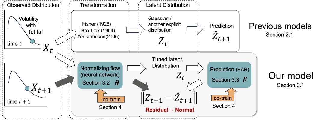
Our approach is demonstrated by the lower half of Figure 1. A volatility value Xt at the timestep t is transformed with a neural network, specifically, a technique of normalizing flow [31]. Normalizing flow realizes an invertible transformation, and it can be trained to acquire the best approximation to a desired distribution. The transformed latent values Z1, ⋅⋅⋅, Zt are fed into a prediction model that outputs the estimate at the following timestep $\hat{Z}_{t+1}$, for which we use a heterogeneous auto-regressive (HAR) model [8]. At the same time, we have the actual realized volatility Xt + 1 of time t + 1, which is transformed into Zt + 1. The residual $\hat{Z}_{t+1}-Z_{t+1}$ can be used to jointly train both the transformation and prediction, naturally realized as an expectation–maximization procedure.
We show how our setting outperforms other possibilities when using no transformation or using analytical or simple neural-network transformations.
2 RELATED WORKS
First proposed in the 1970s [7], with a greater availability of high-frequency data, RV now holds the key to many financial engineering tasks, such as the prediction of return variation [2, 37] and option pricing [9].
This paper focuses on the problem of RV prediction with a distributional transformation. Various analytical functions have been considered previously, which we summarize in Section 2.1. While the transformation operates for each timestep, it requires a time-series model to address the temporal dependence across timesteps. Section 2.2 introduces several such time-series models. Moreover, our approach considers the transformed RV as latent variables; Section 2.3 compares our approach with existing latent-variable models.
2.1 Realized Volatility Prediction with Analytical Transformations
The use of distributional transformations dates back to Fisher [16], where a Student's t variable was expanded as an infinite series of normal variables. In another early work, Wallace [39] proposed a simple approximation form that was found to work exceptionally well transforming between Gaussian and Student's t distributions [28].
A transformation can be used to improve the Gaussianity of a dataset that significantly deviates from a Gaussian distribution. This is often beneficial as Gaussianity occurs as an assumption underlying many statistical and econometric models.
The modern research on distributional transformation for economic data is largely based on Box and Cox [4]’s seminal work, which introduced a family of power transformations now called Box-Cox transformations. Box-Cox transformations include the identity transformation (i.e., f(x) = x) and the log transformation as two special cases. Box-Cox transformations are applied widely, but they only allow positive inputs. Yeo-Johnson transformations [41] were later introduced to generalize Box-Cox to include zero and negative inputs. Apart from power transformations, numerous alternatives have been proposed. Hoyle [23] summarized 18 different analytical transformations. Other choices include the Tukey g-and-h [38], the Lambert W function [19], and exponential functions [40].
While the improvement via a Gaussianizing transformation is frequently observed for cross-sectional data (i.e., a collection of samples at a given time), it does not apply to sequential data. Proietti and Lütkepohl [29] tested Box-Cox transformations on various real datasets with other transformations and found that Box-Cox transformations showed advantages only in a fifth of all cases. Taylor [35] investigated the use of Box-Cox transformations for RV prediction. Among several pre-defined choices of the parameter λ of the Box-Cox transformation, λ = 1/4 performed the best. However, as mentioned in the Introduction, the “correct” shape of the transformed distribution is influenced by the time-series prediction model. The optimal parameter in one scenario might be sub-optimal in other scenarios.
This study uses neural networks for the transformation. Simple neural-network transformations have been considered previously for time-series modeling. Snelson et al. [32] proposed using an additive mixture of tanh functions, a two-layer feed-forward neural network. The parameters in the neural network were restricted to be positive, so that the neural network remains invertible. Recent state-of-the-art techniques are with normalizing flows [13, 31, 34], which provide more powerful choices than the mixture-of-tanh approach in Snelson et al. [32].
2.2 Realized Volatility Prediction Models
Realized volatility, like other volatility measures, exhibits long-memory characteristics often referred to as “volatility clustering” [10]. Based on this finding, many models have been proposed to predict RV, among which two are especially popular. The first is the heterogeneous auto-regressive (HAR) model by Corsi [8], which uses a linear combination of past volatility terms defined over different time periods to predict future volatility. HAR is simple but performs well in practice; therefore, we use it as the prediction model in this paper. The other prevalent model is the auto-regressive fractionally integrated moving average (ARFIMA) [22], which utilizes fractional differencing operators to enable long memory.
It must be noted, however, that RV prediction is closely related to the fat tail problem in financial returns. Research on the fat tails in financial returns dates to Mandelbrot [26] and Fama [15], who noticed that substantial price changes occur more frequently than a Gaussian predicts; thus, the observed return distribution shows a larger kurtosis than a Gaussian (i.e., it has a fat tail). This observation was further validated on large-scale measurements of high-frequency price data [17, 20, 21, 27]. Volatility prediction models have been developed to account for the fat-tailed distribution of returns. But as we will show via baselines in Section 6, this implicit approach via volatility models is often insufficient to fully capture the fat tail.
2.3 Latent Sequential Models
The modeling of a transformed time series can be seen as a kind of latent-variable model. Realized volatilities are “observable” variables while the transformed values are seen as “latent.” Because of the long-memory nature of price time-series, the long-range dependence between the latent variables must be addressed. How to integrate financial econometrics methods into the latent-variable framework of machine learning remains a question.
Several latent-variable methods are considered relevant to our approach. The first is the Kalman filter [24], which assumes that all latent variables are Gaussian and governed by a linear Markovian process. A Kalman filter is estimated by making an initial guess of the earliest latent variable and then progressively gets refined by incorporating new observations at later timesteps.
The second is the hidden Markov models (HMMs) [3]. HMMs are more elaborate latent-variable models that have been used widely in various fields [5]. Kalman filters can be viewed as special cases of HMMs, even though they were studied in different research streams for a long time [5].
Nevertheless, the Markovian nature of Kalman filters and HMMs makes it hard to capture the long memory in RV time-series data [8]. In contrast, a simpler HAR can easily access a timestep far back (e.g., 22 timesteps previous to current), which is much more straightforward than HMMs in incorporating the long memory and has been found to work well.
In this paper, we use normalizing flows (NFs) to assist HAR models in capturing the complex RV distribution. NFs were proposed for variational inference [31], which is a method frequently used for latent-variable modeling. Thus far, normalizing flows have been shown to be effective in various applications, such as density estimation [34], generative modeling [13], variational inference [31], noise modeling [1], and time-series modeling [12].
In a recent work by Deng et al. [12], normalizing flows were used to transform a time series into a Brownian motion. As Brownian motions are Markov processes, the model by Deng et al. [12] can be seen as a hidden Markov model in which the latent Gaussian variables are estimated using a normalizing flow. In contrast, the latent process in this work must capture the long-memory phenomena observed in real RV data [8].
3 REALIZED VOLATILITY PREDICTION VIA TRANSFORMATION
Daily RV is the root sum of quadratic price variations during a trading day. RV measures the amount of financial risk during the day and is calculated using high-frequency price records. Let pt, i denote the i-th high-frequency price of a stock of day t (t = 1, ⋅⋅⋅, T). Then, the daily RV, xt, is calculated as follows:
(1)
The prediction of daily RV is to estimate xt + 1 using the previous values x≤ t ≡ [x1, ⋅⋅⋅, xt]. Let yβ denote a RV prediction model with parameters β. The aim is to find the best parameters that minimize the root-mean-square error (RMSE) between the prediction and the true values, as follows:
(2)
3.1 Prediction with Transformed Time Series
In this paper, we study the task of predicting RVs with a learnable monotonic transformation $f_{\boldsymbol {\theta }}:\mathbb {R}\rightarrow \mathbb {R}$ parameterized by θ. At every timestep t, realized volatility xt is transformed into zt = fθ(xt), which follows a latent distribution. Instead of predicting xt + 1 directly, zt + 1 is predicted as $\hat{z}_{t+1}$ using z≤ t, and the realized volatility xt + 1 is then estimated from $\hat{z}_{t+1}$. The entire prediction procedure is as follows:
(3)
(4)
(5)
Using the transformation fθ has multiple advantages. First, the transformed realized volatilities better approximate Gaussian distributions, an implicit assumption that underlies many prediction models. Thus, the prediction model is estimated with less bias. Second, for a linear prediction model yβ, the use of nonlinear transformation fθ enables capturing nonlinear temporal dependency.
3.2 Normalizing Flow
In this paper, we propose implementing the invertible transformation fθ with normalizing flow, a deep-learning technique. Normalizing flow refers to invertible neural networks for which the inverse can be efficiently computed. Specifically, we use neural ordinary differential equations (NODE) [6], a special kind of normalizing flow.
A NODE is a first-order ordinary differential equation parameterized by a neural network:
(6)
(7)
(8)
3.3 Heterogeneous Auto-Regression
For the prediction model yβ, we use the heterogeneous auto-regressive (HAR) model [8]. HAR is one of the most common models for RV prediction.
HAR is a linear regression model that incorporates RV components during three different periods, as follows:
(9)
Although this paper focuses on HAR, the proposed method can be applied to prediction models other than HAR. Because normalizing flow specifies a wide family of continuous functions, it requires little knowledge about the prediction model to effectuate the prediction in Formulas (3) through (5). The universality of our method with different prediction models remain a future work.
4 CO-TRAINING TRANSFORMATION WITH PREDICTION MODEL
Previously, the estimation of transformation parameters was done prior to that of the prediction model, following some sub-optimal objectives, such as the presumed Gaussianity of the transformed data.
In the following, we propose a method to co-train (i.e., jointly train) the transformation with the prediction model. A primary challenge in this approach arises when the transformation and prediction components employ different techniques, like neural networks and linear regression in our case. Existing literature has yet to present a unified framework that optimizes both components together. This section details our solution to address this challenge.
4.1 Parameter Estimation via Expectation Maximization
Let X = [X1, X2, ⋅⋅⋅] and Z = [Z1, Z2, ⋅⋅⋅] denote the random processes underlying the raw and the transformed realized volatilities, respectively, where Zs = fθ(Xs) (s = 1, 2, ⋅⋅⋅). The normalizing flow fθ is optimized subject to a maximum-likelihood objective as follows:
(10)
(11)
(12)
(13)
In this work, the dependence of Zt on Xt is deterministic via the normalizing flow, while that of Xt + 1 on Zt can be random. Hence, the sampling procedure of Z ∼ P(· ∣X, θ(i)) in Formula (13) is simply to apply fθ to every timestep of X1, X2, ⋅⋅⋅, and the expectation average is taken over the RV time series of multiple stocks. On the other hand, the term within the expectation operation of Formula (13) decomposes into the following due to the change-of-variable theorem:
(14)
(15)
Notice that in Formula (15), P(Zs + 1∣Z≤ s) represents the prediction model yβ applied to the latent process, and it does not specify how the parameters β should be estimated. Therefore, optimization of the parameters in the prediction model (i.e., β) can be effectuated via a different objective function from that in Formula (13). This is important because HAR and many other financial time-series models are conventionally estimated with a least-square objective function, which imposes a weaker assumption on the distribution of residuals and often shows better robustness. The probability density P(Zs + 1∣Z≤ s) is obtained via an estimation, which is detailed in Section 4.2.
Hence, the co-training procedure of fθ and yβ is via iterative updates as follows: at each iteration, the sampling step Z ∼ P(· ∣X, θ(i)) in Formula (13) is conducted as a random sampling of X≤ t from the RV time series of stocks and then transforming X≤ t into Z≤ t. Using the samples of Z≤ t, the parameters of the prediction model (i.e., β) can be estimated via any adequate method; here for HAR, we used the Python package arch 1 to estimate β. Then, Zt + 1 is predicted, and the expectation of log-likelihoods log P(xt + 1∣Z≤ t, θ) is calculated using Formula (15). Finally, the $\mathop{arg\,max}$ operation in Formula (13) is approximated by a mini-batch gradient ascent step over the expectation of the log-likelihoods.
4.2 Residual Density Estimation
The conditional probability density P(Zs + 1∣Z≤ s) is determined by the prediction model yβ, which produces an estimate $\hat{Z}_{s+1} = y_{\boldsymbol {\beta }}(Z_{\le s})$ based on previous latent states. Thus, the conditional probability density is equivalent to the density of the prediction residual:
(16)
The distributions of residuals are usually unknown in practice. In this paper, we assume they are Gaussian. This assumption could be inappropriate if the prediction is with the raw RV or when the transformation fθ is as simple as a Box-Cox transformation [29]. Nevertheless, we find empirically that a Gaussian distribution is a good approximate for the residuals after the normalizing flow is optimized, which could be due to the larger capacity of the normalizing-flow neural network. In addition, we assume the residuals to be homogeneous across time (i.e., ɛs follows the same Gaussian distribution for every timestep s). Using a more advanced time-series model would improve the homogeneity of the residuals, which is left to future work.
Therefore, the residuals ɛs ∼ N(μ, v) (s = 1, 2, ⋅⋅⋅, t), where μ and v are the mean and variance of the Gaussian distribution. μ is set to zero2 and v is estimated as the empirical variance: $v = \left(\sum _{s=1}^t (\varepsilon _s - \mu)^2 \right) / (t-1)$. Notice that v involves the whole period 1, 2, ⋅⋅⋅, t, but is used for calculating P(ɛs + 1∣Z≤ s) for s < t, which means the calculation involves “further information” at timestep s < t. Nevertheless, it does not invalidate our approach because the calculation of P(ɛs + 1∣Z≤ s) is only required in parameter estimation; that is, making out-of-sample prediction on Zt + 1, Zt + 2, ⋅⋅⋅ does not involve the calculation of P(ɛs + 1∣Z≤ s).
5 EXPERIMENT
5.1 Data
The proposed method is evaluated on a dataset of 100 major stocks listed on the New York Stock Exchange. The dataset covers a continuous time period of 480 trading days from December 1st, 2015, to October 25th, 2017. The daily RV values were calculated according to Formula (1) for every stock. Thus, 100 RV time series of 480 timesteps were acquired. In computing the daily RV, we followed Corsi [8] and did not include the overnight price variation. That is, we did not include $p_{t+1,1} - p_{t, n_t}$ in the summation of Formula (1), where nt denotes the number of high-frequency prices within day t as mentioned in Section 3.1.
In this paper, the RV of a day is calculated with high-frequency prices that are recorded every five minutes. That is, pt, i + 1 was taken five minutes later than pt, i. The value of high-frequency price is calculated as the mid-price [33] of the order book, which is an average of the highest bid price and the lowest ask price weighted by their volumes, as follows:
(17)
(18)
5.2 Settings
The RV time series were split into training, validation, and test sets chronologically, at a ratio of 300, 60, and 120 days.
We conducted the experiments in a univariate time-series setting by viewing all 100 RV time series as independent samples drawn from the same random process X1, X2, ⋅⋅⋅. Thus, this accommodates the notion of taking an expectation over IID samples in Formula (13). The normalizing flow fθ was optimized on the training set (i.e., the first 300 days of the RV history of all stocks). Using an Adam [25] optimizer, we conducted 200 iterations of parameter updates and evaluated the model on the validation set at every five training iterations, thus producing 40 different snapshots of parameters. The snapshot that achieved the highest log-likelihood in Formula (15) was regarded as the best. In the following, we report the performance of this best snapshot on the test set.
For the neural network NNθ used in the NODE (see Formula (6)), we used a simple multi-layer perceptron with two hidden layers. Each hidden layer had four hidden units. Formally,
(19)
(20)
| Transformation |
|
Out-of-sample prediction | In-sample residual Gaussianity | ||||
|---|---|---|---|---|---|---|---|
| RMSE | Percentage of best | R2 | Skewness | ||||
| Identity | Gaussian | 0.5695*** | 10% | 93.22 | 1.788 | ||
| Wallace's | Gaussian | 0.5660** | 19% | 98.12 | 0.7010 | ||
| Yeo-Johnson | Gaussian | 0.5627* | 2% | 99.09 | 0.2752 | ||
| tanh(1) | Gaussian | 0.5642** | 6 % | 99.31 | 0.2059 | ||
| tanh(5) | Gaussian | 0.5636** | 6 % | 99.11 | 0.2141 | ||
| tanh(10) | Gaussian | 0.5638** | 11 % | 99.20 | 0.1693 | ||
| Our approach | |||||||
| NODE(τ =5.00) | Gaussian | 0.5630 | - | 99.14 | 0.2141 | ||
| NODE(τ =0.25) | Gaussian | 0.5620 | 46% | 98.81 | 0.3928 | ||
5.3 Baselines
We considered different baseliens by varying the transformation fθ and the distribution for the residuals ɛs (see Formula (9)).
For alternative transformations, we considered the following:
- transformation: fθ(x) = x, which is equivalent to not applying a transformation.
- transformation [39]:
where θ = {d}.\begin{equation} f_{\boldsymbol {\theta }}(x)= \pm \frac{8d+1}{8d+3}\sqrt {d\log (1+|x|^2/d)}, \end{equation}
(21) - transformation [41]: a generalization of the Box-Cox transformation [4] to allow non-positive inputs, defined as follows:
where θ = {λ}.\begin{equation} f_{\boldsymbol {\theta }}(x) = \left\lbrace \begin{array}{ll}((x+1)^\lambda - 1) / \lambda & \text{if}~\lambda \ne 0, x\ge 0, \\ \log (x+1) & \text{if}~\lambda =0, x\ge 0, \\ -((-x+1)^{(2-\lambda)} - 1) / (2 - \lambda) & \text{if}~\lambda \ne 2, x< 0, \\ -\log (-x+1) & \text{if}~\lambda =2, x< 0, \end{array}\right. \end{equation}
(22) - transformation [32]: a simplest neural network with a single hidden layer, defined as follows:
where $\boldsymbol {\theta }=\bigcup _{i=1}^k \lbrace u_i, v_i, b_i\rbrace$. For fθ to be invertible, ui, vi (i = 1, ⋅⋅⋅, k) are restricted to be positive.\begin{equation} f_{\boldsymbol {\theta }}(x) = \sum _{i=1}^k u_i \tanh (v_i x+b_i), \end{equation}
(23)
As for the distribution of the residuals, we tested the generalized Student's t distribution (in addition to the Gaussian by default), which is defined by the following probability density function with mean μ, variance v, and d degrees of freedom:
(24)
6 RESULTS
6.1 Prediction Accuracy
Table 1 summarizes the overall results over the dataset of 100 stocks acquired with different transformations. Each row represents a transformation. Our transformation via normalizing flow is shown at the bottom of the table. The third and fourth columns show the scores concerning HAR prediction accuracy. RMSE was used as the primary evaluation metric to follow the previous works [8]. A smaller RMSE implies a higher precision.
The third column of Table 1 reports the average RMSE (mean value) over the 100 stocks. One-tailed t-tests were conducted to assess the statistical significance of our method (NODE with τ = 0.25) compared with the other transformations, assuming the null hypothesis that the mean improvement in RMSE is equal to zero. Asterisks (*) in the third column indicate statistical significance: * (p < 0.05), ** (p < 0.01), *** (p < 0.001). The fourth column shows the proportion of stocks on which a method achieved the lowest RMSE, or “percentage of the best.” The best scores are indicated in bold, and the second-best scores are underlined. For a robustness test, we also examined NODE with τ = 5.00 which has excessive complexity as a transformation; we omitted the p-value and the “percentage of the best” value as it serves merely as a robustness test.
Our approach (bottom row) achieved the lowest RMSE score at 0.5620, a clear improvement of 0.0075 compared with the identity transformation that scored 0.5695. The second-best at 0.5627 was the Yeo-Johnson transformation, which is a common way of preprocessing non-Gaussian data in practice; nevertheless, our method still outperformed the Yeo-Johnson transformation. Compared with the baseline transformations, the improvements of NODE in RMSE are statistically significant at the 5% (Yeo-Johnson), 1% (Wallace's and tanh transformations), and 0.1% (Identity) levels. With respect to the “percentage of the best,” the advantage of NODE is more evident. NODE achieved the lowest RMSE on 46 of the 100 stocks; in comparison, the Yeo-Johnson transformation won on only two stocks.
The significant margin between NODE and Yeo-Johnson on the “percentage of the best” is interesting, in contrast to their relatively close performance in average RMSE. This indicates that on many stocks, NODE and Yeo-Johnson transformed realized volatilities into close distributions, but NODE performed slightly better in most cases. While power transformations like Yeo-Johnson are careful choices made by practitioners after decades, NODE was learned from data. However, NODE “discovered” the power transformations were the best choices and further improved over them.
The transformations denoted by tanh(k) (k = 1, 5, 10) are the simplest feed-forward neural networks, and k represents the number of hidden units. When k was increased from 1 to 5, the average RMSE was improved from 0.5642 to 0.5636. However, when k was further increased to 10, the score degraded to 0.5638.
The degradation at large k values might be caused by the increased risk of overfitting to the training set. The tanh transformations with a large k or NODE with a large τ had a stronger approximation capability, but they overfitted to the training set. Evidence of this is that on 29 stocks, simpler transformations, including Identity or Wallace's, had the best RMSE. On these stocks, the data distribution of the test set shows inconsistency with the training set, which is common in a financial market that is a non-stationary system. Such overfitting is also seen for NODE when τ was increased from 0.25 to 5.00 when RMSE increased from 0.5620 to 0.5630.
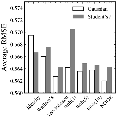
As an ablation analysis, we evaluated the robustness of the presumption made in Section 4.2 that the residuals of HAR (i.e., ɛs in Formula (9)) follow a Gaussian distribution. Instead of assuming that ɛs ∈ N(μ, v), the ablated version assumes a generalized Student's t distribution with an additional parameter d denoting the degrees of freedom. Note that d → ∞ recovers a Gaussian distribution.
Figure 2 shows the average RMSE scores (vertical axis) when the residual distribution was assumed to be either Gaussian (white bars) or generalized Student's t (grey bars) grouped by the transformation fθ. When the residuals are assumed to follow a generalized Student's t distribution, the probability density in Equation (16) is determined using the PDF of the Student's t distribution, instead of the Gaussian PDF. Consequently, the transformation parameters θ that are estimated yield an RMSE score that differs from what would be expected under a Gaussian residual assumption.
In Figure 2, the white bars are the values in Table 1 in the third column. Except for the Identity transformation, we observed increased RMSE scores when the presumed distribution was a Student's t, which means a decrease in prediction accuracy. The largest increase in RMSE is observed with the tanh(1) transformation, implying tanh(1) to be sensitive to the distributional assumption. In contrast, NODE still achieved the smallest RMSE score at 0.5643, the same as with a Yeo-Johnson transformation. The results in Figure 2 suggest the robustness of our approach even under a generalized Student's t distribution assumption for residuals that is not optimal.
6.2 Qualitative Comparison
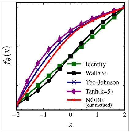
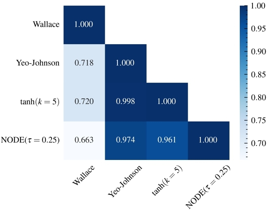
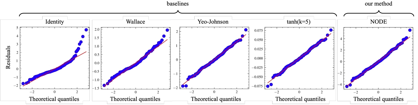
Figure 3 provides a comparison between the distribution of residuals ɛs defined in Formula (9) (vertical axes) and the standard normal distribution (horizontal axes) for the stock “BABA” (i.e., the Q-Q plot). Each plot represents a different transformation listed in Section 5.3. In each plot, a point represents the residual at a timestep; the vertical axis shows the residual values, and the horizontal axis shows the theoretical percentiles if the residuals follow a standard normal distribution. The straight red line is a linear fit of the points, and a better fit implies a higher degree to which the residuals follow a Gaussian distribution.
As seen in the first plot of Figure 3 (Identity transformation), the residuals of the raw RV deviate from the linear fit at large positive quantiles. This shows how HAR fails to fully capture the skewness in RV time series. In contrast, with a transformation, the Gaussianity of the residuals was largely improved. This improvement is visible for all the transformations shown in Figure 3. Among the transformations tested, the Yeo-Johnson, the tanh(5), and NODE produced impressive Gaussianity, and they are indistinguishable within a large range.
The Gaussianity of the residuals is further quantified using two metrics, as shown in the two right-hand columns in Table 1. The first metric is the R2 score of the linear fit in the Q-Q plots of Figure 3, and the other is the skewness (i.e., the third moment) of the residuals. The two right-hand columns present the average R2 and the average skewness over the 100 stocks.
Consistent with the observation of Figure 3, without a transformation (first row), HAR produced residuals with a low R2 at 93.22% and a high skewness at 1.7883, implying poor Gaussianity. The Gaussianity was greatly improved by using a transformation. R2 was improved to 99.14%, and skewness was reduced to 0.2141 with a NODE having τ = 5.00 (second to last row).
When R2 exceeds 99%, an improvement in R2 or a reduction in skewness did not translate into an improvement in out-of-sample RMSE. This corresponds with our previous conjecture on overfitting. Nevertheless, even with the same level of R2 and skewness, NODE with τ = 5.00 still outperformed the tanh(5) transformation in out-of-sample RMSE.
Figure 4 provides a visualized comparison between the transformations on the real line. The horizontal axis represents the input $x\in \mathbb {R}$ to the transformation fθ, and the vertical axis shows the output (i.e., fθ(x)). Note that the realized volatilities were z-score standardized in preprocessing, which produced negative x. For visualization, we also linearly rescaled the transformations so that fθ(− 2) = −2 and fθ(2) = 2. As HAR is a linear model with a bias term, the estimation and prediction with HAR are invariant under linear rescaling to the transformation.
Each curve in Figure 4 represents a transformation. The straight green line represents the identity function, and the dotted red plot represents the NODE transformation. The NODE, Yeo-Johnson (in blue), and tanh transformations (in purple) all showed a concave shape: their slopes gradually decrease as x increases. This corresponds with our expectation that larger realized volatilities are calibrated more than smaller realized volatilities to eliminate skewness.
At large x, NODE showed almost perfect consistency with the Yeo-Johnson transformation. However, a discrepancy is seen at small x where NODE grows linearly, similar to the Identity function. In other words, NODE viewed it “unnecessary” to apply nonlinear calibration to small realized volatilities. With the Yeo-Johnson or tanh transformations, such local linear growth is not possible, as power and tanh transformations are defined globally over the real line.
Figure 5 presents the Pearson's correlation coefficients between the transformations on the RMSE improvements over the Identity transformation, measured for the 100 stocks. The RMSE values were obtained through out-of-sample evaluations, and the mean value for each transformation has been reported in Table 1, in the third column.
These correlation results align closely with the graph of fθ(x) in Figure 4. Notably, the Yeo-Johnson and the tanh (k = 5) transformations exhibit a correlation coefficient of 0.998. This is unsurprising as they appear nearly identical in shape in Figure 4 (the purple and blue plots). Furthermore, NODE also demonstrates a high correlation with the Yeo-Johnson transformation, which validates our conjecture in Section 6.1 that NODE has “discovered” (while also outperformed) power transformations from the data.
7 CONCLUSION
We proposed a new method to enhance the prediction of realized voltility by co-training a simple linear prediction model with a nonlinear transformation. In contrast to previous methods that estimate the transformation before the prediction model and use separate objective functions at the two steps, we propose to co-train the two parts following a unified maximum-likelihood objective function. Additionly, we introduced a method based on the expectation-maximization algorithm to jointly estimate the parameters for both parts.
For the nonlinear transformation, we incorporated normalizing flows which represent the state-of-the-art in neural distributional transformations. We demonstrated how the proposed co-training procedure can utilize complex transformations, a task challenging for prior methods restricted to simple analytical functions.
On a dataset of the high-frequency price history of 100 stocks for two years (2015-2017), the proposed method significantly outperformed predictions with the raw time series in average RMSE. Compared with analytical and neural-network baselines, our method achieved the best RMSE on 46 of the 100 stocks, suggesting its effectiveness and robustness.
ACKNOWLEDGMENTS
This work was supported by JSPS KAKENHI Grant Numbers JP20K20492 and JP21H03493.
REFERENCES
- Abdelrahman Abdelhamed, Marcus A Brubaker, and Michael S Brown. 2019. Noise flow: Noise modeling with conditional normalizing flows. In Proceedings of the IEEE/CVF International Conference on Computer Vision. 3165–3173.
- Torben G Andersen, Tim Bollerslev, Francis X Diebold, and Paul Labys. 2000. Exchange rate returns standardized by realized volatility are (nearly) Gaussian.
- Leonard E Baum and Ted Petrie. 1966. Statistical inference for probabilistic functions of finite state Markov chains. The annals of mathematical statistics 37, 6 (1966), 1554–1563.
- George EP Box and David R Cox. 1964. An analysis of transformations. Journal of the Royal Statistical Society Series B: Statistical Methodology 26, 2 (1964), 211–243.
- Olivier Cappé, Eric Moulines, and Tobias Rydén. 2005. Inference in hidden Markov models. Springer, New York ; London. OCLC: ocm61260826.
- Ricky TQ Chen, Yulia Rubanova, Jesse Bettencourt, and David K Duvenaud. 2018. Neural ordinary differential equations. Advances in neural information processing systems 31 (2018).
- Peter K Clark. 1973. A subordinated stochastic process model with finite variance for speculative prices. Econometrica: journal of the Econometric Society (1973), 135–155.
- Fulvio Corsi. 2009. A simple approximate long-memory model of realized volatility. Journal of Financial Econometrics 7, 2 (2009), 174–196.
- Fulvio Corsi, Nicola Fusari, and Davide La Vecchia. 2013. Realizing smiles: Options pricing with realized volatility. Journal of Financial Economics 107, 2 (2013), 284–304.
- Fulvio Corsi, Stefan Mittnik, Christian Pigorsch, and Uta Pigorsch. 2008. The volatility of realized volatility. Econometric Reviews 27, 1-3 (2008), 46–78.
- Arthur P Dempster, Nan M Laird, and Donald B Rubin. 1977. Maximum likelihood from incomplete data via the EM algorithm. Journal of the royal statistical society: series B (methodological) 39, 1 (1977), 1–22.
- Ruizhi Deng, Bo Chang, Marcus A Brubaker, Greg Mori, and Andreas Lehrmann. 2020. Modeling continuous stochastic processes with dynamic normalizing flows. Advances in Neural Information Processing Systems 33 (2020), 7805–7815.
- Laurent Dinh, David Krueger, and Yoshua Bengio. 2015. NICE: Non-linear Independent Components Estimation. In 3rd International Conference on Learning Representations, ICLR 2015, San Diego, CA, USA, May 7-9, 2015, Workshop Track Proceedings, Yoshua Bengio and Yann LeCun (Eds.). http://arxiv.org/abs/1410.8516
- Robert F Engle. 1982. Autoregressive conditional heteroscedasticity with estimates of the variance of United Kingdom inflation. Econometrica: Journal of the econometric society (1982), 987–1007.
- Eugene F Fama. 1965. The behavior of stock-market prices. The journal of Business 38, 1 (1965), 34–105.
- Ronald A Fisher. 1926. Expansion of “student's” integral in powers of n− 1. Metron 5 (1926), 109–112.
- Xavier Gabaix, Parameswaran Gopikrishnan, Vasiliki Plerou, and H Eugene Stanley. 2003. A theory of power-law distributions in financial market fluctuations. Nature 423, 6937 (2003), 267–270.
- DK Ghaddar and H Tong. 1981. Data transformation and self-exciting threshold autoregression. Journal of the Royal Statistical Society Series C: Applied Statistics 30, 3 (1981), 238–248.
- Georg M Goerg. 2015. The lambert way to gaussianize heavy-tailed data with the inverse of Tukey's h transformation as a special case. The Scientific World Journal 2015 (2015).
- Parameswaran Gopikrishnan, Martin Meyer, LA Nunes Amaral, and H Eugene Stanley. 1998. Inverse cubic law for the distribution of stock price variations. The European Physical Journal B-Condensed Matter and Complex Systems 3, 2 (1998), 139–140.
- Parameswaran Gopikrishnan, Vasiliki Plerou, Luis A Nunes Amaral, Martin Meyer, and H Eugene Stanley. 1999. Scaling of the distribution of fluctuations of financial market indices. Physical Review E 60, 5 (1999), 5305.
- Clive WJ Granger and Roselyne Joyeux. 1980. An introduction to long-memory time series models and fractional differencing. Journal of time series analysis 1, 1 (1980), 15–29.
- Mike H Hoyle. 1973. Transformations: An introduction and a bibliography. International Statistical Review/Revue Internationale de Statistique (1973), 203–223.
- Rudolph E Kalman and Richard S Bucy. 1961. New results in linear filtering and prediction theory. Journal of Basic Engineering 83, 1 (1961), 95–108.
- Diederik P Kingma and Jimmy Ba. 2014. Adam: A method for stochastic optimization. arXiv preprint arXiv:1412.6980 (2014).
- B. Mandelbrot. 1963. The Variation of Certain Speculative Prices. The Journal of Business 36 (1963), 371–418.
- Vasiliki Plerou, Parameswaran Gopikrishnan, Luis A Nunes Amaral, Martin Meyer, and H Eugene Stanley. 1999. Scaling of the distribution of price fluctuations of individual companies. Physical review e 60, 6 (1999), 6519.
- P Prescott. 1974. Normalizing transformations of Student's t distribution. Biometrika 61, 1 (1974), 177–180.
- Tommaso Proietti and Helmut Lütkepohl. 2013. Does the Box–Cox transformation help in forecasting macroeconomic time series?International Journal of Forecasting 29, 1 (2013), 88–99.
- Prajit Ramachandran, Barret Zoph, and Quoc V. Le. 2018. Searching for Activation Functions. In 6th International Conference on Learning Representations, ICLR 2018, Vancouver, BC, Canada, April 30 - May 3, 2018, Workshop Track Proceedings. OpenReview.net. https://openreview.net/forum?id=Hkuq2EkPf
- Danilo Rezende and Shakir Mohamed. 2015. Variational inference with normalizing flows. In International conference on machine learning. PMLR, 1530–1538.
- Edward Snelson, Zoubin Ghahramani, and Carl Rasmussen. 2003. Warped gaussian processes. Advances in neural information processing systems 16 (2003).
- Sasha Stoikov. 2018. The micro-price: a high-frequency estimator of future prices. Quantitative Finance 18, 12 (2018), 1959–1966.
- Esteban G Tabak and Eric Vanden-Eijnden. 2010. Density estimation by dual ascent of the log-likelihood. Communications in Mathematical Sciences 8, 1 (2010), 217–233.
- Nick Taylor. 2017. Realised variance forecasting under Box-Cox transformations. International Journal of Forecasting 33, 4 (2017), 770–785.
- SJ Taylor. 1982. Financial returns modelled by the product of two stochastic processes-A study of the daily sugar prices 1961-75. Time Series Analysis: Theory and Practice 1 (1982), 203–226.
- Dimitrios D Thomakos and Tao Wang. 2003. Realized volatility in the futures markets. Journal of empirical finance 10, 3 (2003), 321–353.
- John W Tukey. 1977. Modern techniques in data analysis. In Proceedings of the NSF-Sponsored Regional Research Conference, Vol. 7. Southern Massachusetts University North Dartmouth, MA, USA.
- David L Wallace. 1959. Bounds on normal approximations to Student's and the chi-square distributions. The Annals of Mathematical Statistics (1959), 1121–1130.
- Xing Yan, Weizhong Zhang, Lin Ma, Wei Liu, and Qi Wu. 2018. Parsimonious quantile regression of financial asset tail dynamics via sequential learning. Advances in neural information processing systems 31 (2018).
- In-Kwon Yeo and Richard A Johnson. 2000. A new family of power transformations to improve normality or symmetry. Biometrika 87, 4 (2000), 954–959.
FOOTNOTE
1 https://github.com/bashtage/arch
2One may alternatively relax the prior of μ = 0 and set μ to be empirical mean instead; however, we did not observe improvements by doing so, as the empirical mean is usually close to zero.
Permission to make digital or hard copies of all or part of this work for personal or classroom use is granted without fee provided that copies are not made or distributed for profit or commercial advantage and that copies bear this notice and the full citation on the first page. Copyrights for components of this work owned by others than the author(s) must be honored. Abstracting with credit is permitted. To copy otherwise, or republish, to post on servers or to redistribute to lists, requires prior specific permission and/or a fee. Request permissions from permissions@acm.org.
ICAIF '23, November 27–29, 2023, Brooklyn, NY, USA
© 2023 Copyright held by the owner/author(s). Publication rights licensed to ACM.
ACM ISBN 979-8-4007-0240-2/23/11…$15.00.
DOI: https://doi.org/10.1145/3604237.3626870