TRAQID - Traffic-Related Air Quality Image Dataset
DOI: https://doi.org/10.1145/3702250.3702260
ICVGIP 2024: Indian Conference on Computer Vision Graphics and Image Processing, Bengaluru, India, December 2024
Air quality estimation through sensor-based methods is widely used. Nevertheless, their frequent failures and maintenance challenges constrain the scalability of air pollution monitoring efforts. Recently, it has been demonstrated that air quality estimation can be done using image-based methods. These methods offer several advantages including ease of use, scalability, and low cost. However, the accuracy of these methods hinges significantly on the diversity and magnitude of the dataset utilized. The advancement of air quality estimation through image analysis has been limited due to the lack of available datasets. Addressing this gap, we present TRAQID - Traffic-Related Air Quality Image Dataset, a novel dataset capturing 26,678 front and rear images of traffic alongside co-located weather parameters, multiple levels of Particulate Matters (PM) and Air Quality Index (AQI) values. Spanning over multiple seasons, with over 70 hours of data collection in the twin cities of Hyderabad and Secunderabad, India, the TRAQID offers diverse day and night imagery amid unstructured traffic conditions, encompassing six AQI categories ranging from “Good” to “Severe”. State-of-the-art air quality estimation techniques, which were trained on a smaller and less-diverse dataset, showed poor results on the dataset presented in this paper. TRAQID models various uncertainty types, including seasonal changes, unstructured traffic patterns, and lighting conditions. The information from the two views (front and rear) of the traffic can be combined to improve the estimation performance in such challenging conditions. As such, the TRAQID serves as a benchmark for image-based air quality estimation tasks and AQI prediction, given its diversity and magnitude. Dataset Link
ACM Reference Format:
Om Rajendra Kathalkar, Nitin Nilesh, Sachin Chaudhari, and Anoop Namboodiri. 2024. TRAQID - Traffic-Related Air Quality Image Dataset. In Indian Conference on Computer Vision Graphics and Image Processing (ICVGIP 2024), December 13--15, 2024, Bengaluru, India. ACM, New York, NY, USA 10 Pages. https://doi.org/10.1145/3702250.3702260
1 Introduction
Air pollution poses a significant global health concern, with air quality deteriorating due to emissions from stationary and mobile sources [36]. Traffic-related pollution significantly deteriorates ambient air quality, emphasizing the crucial importance of monitoring air quality in these areas [3, 37]. The Air Quality Index (AQI), a metric ranging from 0 to 500, provides a measure of air quality, with lower values indicating better air quality and higher values indicating worse air quality. The AQI is determined based on various pollutants such as particulate matter (PM2.5 and PM10), which are minute solid or liquid particles suspended in the air, measured in μg/m3, along with other gaseous pollutants. Particularly in India, the overall air quality is mainly degraded due to PM2.5 and PM10 [16]. The Central Pollution Control Board (CPCB), India [14] has set up pollution monitoring stations across various cities to monitor air quality. These stations have expensive monitoring instruments and equipment to measure various atmospheric parameters. However, many of these stations are too far apart to capture local pollution events effectively. For instance, in the twin cities of Hyderabad and Secunderabad, which cover an area of 650 km2, there are only 14 CPCB stations1. According to [28], pollution levels fluctuate every 300-500 meters due to the diverse nature of Indian cities. This sparse distribution fails to provide the necessary granularity for reliable air quality monitoring across the urban landscape. Furthermore, these stations capture data points at 15-minute intervals, which is insufficient for real-time air quality assessment.
As a solution, many cities have deployed devices with low-cost PM sensors to address this issue, but they often require frequent maintenance and can be unreliable [2, 28]. While these low-cost sensors offer improved spatial coverage, they present significant challenges when scaled to city-wide deployment, particularly in large Indian urban centers. The sheer size of these cities, combined with the high density of pollution sources, necessitates an extensive network of sensors. This approach incurs substantial costs in terms of device maintenance, calibration, and replacement, making it economically and logistically challenging to implement and sustain over time. Image-based algorithms offer a cost-effective alternative, providing higher spatial and temporal resolution for air quality monitoring. However, the scarcity of comprehensive image-based air quality datasets hinders progress in developing robust and scalable solutions for this critical environmental challenge.
1.1 Image-Based PM Estimation Model
PM in air affects optical images primarily through light scattering, including Rayleigh and Mie scattering [20]. This interaction is described by the Beer-Lambert law:
(1)
(2)
In this equation, I represents the observed hazy image, t is the transmission from scene to camera, J denotes scene radiance, and A is the airlight color vector. The first term, t(x, y)J(x, y), represents direct transmission of scene radiance to the camera, while the second term, (1 − t(x, y))A, describes airlight - ambient light scattered by air molecules and PM into the camera. This model assumes constant atmospheric and lighting conditions, although these factors may vary with weather, solar position, time of day, and season. Moreover, both J and A are influenced not only by meteorological conditions and solar position but also by PM distribution and concentration.
Color information plays a crucial role in PM estimation based on light scattering principles. Rayleigh scattering, predominant when particles are significantly smaller than the wavelength of light, exhibits strong wavelength dependence (λ− 4), contributing to the sky's blue appearance. Conversely, Mie scattering occurs when particle sizes are comparable to light wavelengths, producing a white glare around the sun in particulate-laden air. The combined effects of Rayleigh and Mie scattering modulate the brightness and color saturation of outdoor images. Consequently, color and brightness information encapsulate particle concentration and size data, serving as distinctive features for PM estimation. This relationship between optical characteristics and atmospheric particulate content forms the basis for image-based air quality assessment methodologies.
| Dataset | Multiple View |
|
|
|
|
|
|
|
|
||||||||||||||||
|---|---|---|---|---|---|---|---|---|---|---|---|---|---|---|---|---|---|---|---|---|---|---|---|---|---|
| Mondal et al. [22] | ✘ | ✘ | ✘ | ✘ | ✘ | NA | ✔ | ✔ | 1818 | ||||||||||||||||
| Liu et al. [19] | ✘ | ✘ | ✘ | ✘ | ✔ | NA | ✘ | ✔ | 6587 | ||||||||||||||||
| NWNU-AQI [38] | ✘ | ✘ | ✘ | ✘ | ✔ | NA | ✘ | ✘ | 1241 | ||||||||||||||||
| Nilesh et al. [25] | ✘ | ✘ | ✔ | ✘ | ✔ | ✔ | ✔ | ✘ | 5048 | ||||||||||||||||
| Kow et al. [17] | ✘ | ✔ | ✘ | ✘ | ✘ | NA | ✘ | ✘ | 3549 | ||||||||||||||||
| KHI-AQI [1] | ✘ | ✘ | ✘ | ✘ | ✘ | NA | ✘ | ✘ | 1001 | ||||||||||||||||
| TRAQID (Ours) |
|
✔ | ✔ | ✔ | ✔ | ✔ | ✔ |
|
26678 |
1.2 Related Work
Limited efforts have been devoted to predicting AQI using image-based methods, particularly in the aftermath of the COVID-19 pandemic, with a surge in research activity in this field. Prominent companies such as Google [27], Microsoft [32], IBM [24], and others have been actively engaged in this domain, employing advanced machine learning techniques to monitor air pollution. Researchers globally utilize images captured from stationary or mobile sources to analyze PM concentrations (PM2.5 and PM10) and predict AQI [15, 17, 19, 22, 25, 38]. However, most of the research in this field relies on custom datasets tailored to specific studies.
Dataset: Liu et al.[19] gathered 6587 images from three cities, Beijing and Shanghai in China and Phoenix in the U.S., from fixed scenes. The corresponding PM2.5 data was obtained from local U.S. consulates, while weather and geographical data for the three cities were sourced from online websites. Kow et al.[17] gathered 3549 images taken in Kaohsiung, Taiwan, accompanied by corresponding air quality data, including PM2.5, PM10, and AQI, retrieved from nearby air quality monitoring stations. The dataset includes images captured during both daytime and nighttime. Zhang et al.[38] collected a total of 1241 sky images from a stationary location in Lanzhou, China, spanning from 2018 to 2019, and collected corresponding PM2.5, PM10 and gaseous pollutants data from the nearby monitoring station. In recent studies, Nilesh et al.[25] curated a dataset comprising 5048 images captured from roads of Hyderabad, India using a vehicular setup. Each image was paired with corresponding weather data and PM values obtained from sensors. The data collection occurred over two distinct seasons within a single year. Mondal et al.[22] used images captured from smartphone cameras to predict PM2.5 concentration. They collected a custom dataset comprising 1818 images captured within Dhaka, Bangladesh, spanning from 2020 to 2022. The PM2.5 concentration data corresponding to the images was obtained from the local US consulate, which releases hourly updates of the AQI. However, the dataset lacks features such as temperature and humidity, which play an effective role in determining the air quality.
AQI Estimation: Using either custom-collected or publicly available datasets, many researchers have used traditional and advanced deep learning methods to estimate the AQI and PM values. Liu et al.[19] utilized light attenuation and color information as significant image features for estimating PM levels from images. Additionally, machine learning models were employed to predict PM2.5 values. Mondal et al.[22] utilized a custom-made CNN model with a total of 4.8 million parameters, featuring a single neuron in the final fully connected layer, to predict the PM2.5 value. Kalajdjieski et al.[15] employed a multimodal approach, combining InceptionV3 [35] for image features and an MLP for weather data features. They extended the Inception architecture with a new sub-model path processing weather data through a three-layered MLP. The MLP output is concatenated with the Inception model's output in the final fully connected layer, feeding into a softmax layer to predict the AQI category. Zhang et al.[38] presented AQC-Net, a deep convolutional neural network model based on ResNet [13], aimed at classifying AQI categories. They integrated a self-supervision module called the Spatial and Context Attention block (SCA) into the ResNet18 architecture. This addition enabled encoding of broader scenes into local features and aggregation of spatial context information to enhance specific scene details within each channel. Nilesh et al.[25] employed a combination of deep learning and machine learning methods to predict AQI categories. They utilized YOLOv5 [8] to identify vehicles contributing to pollution in input images. A visibility metric was computed using BRISQUE [21] to assess image clarity. Image features (vehicle count and visibility score) were concatenated with weather features (temperature and humidity) to create feature vectors for each sample. Subsequently, a Random Forest (RF) [4] was trained to classify images into various AQI categories.
1.3 Contribution
We introduce TRAQID - Traffic-Related Air Quality Image Dataset, designed for predicting AQI through image analysis. Our key contributions are:
1) The TRAQID dataset, comprising 26,678 samples from 70 hours of video capture, is the first of its kind to feature both front and rear traffic scene images alongside co-located sensor data. It uniquely combines vehicular traffic observations with essential environmental parameters such as temperature, relative humidity, and PM concentrations. This comprehensive approach captures the variability in urban environments, including diverse traffic patterns, building structures, and geographical features, providing a rich resource for analyzing the interplay between traffic dynamics and air quality.
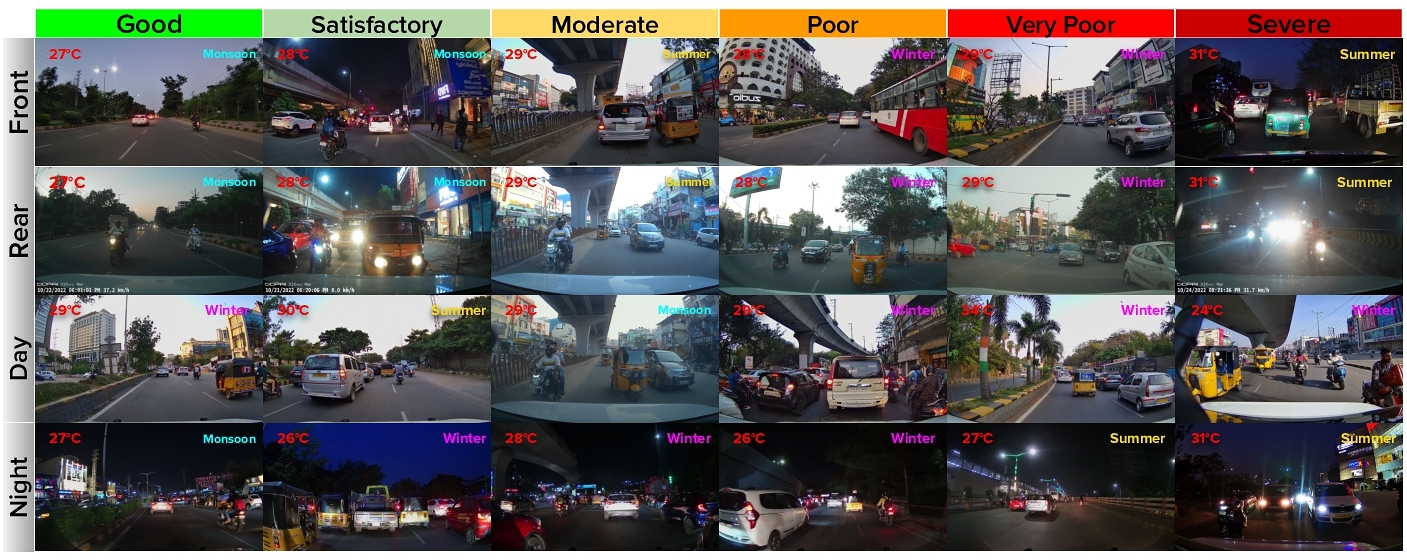
2) The dataset incorporates AQI measurements categorized into six distinct ranges from “Good” to “Severe”, aligning with the classification schema outlined by the CPCB, India. It comprises a diverse collection of images containing both day and night settings across three primary seasons - Summer, Monsoon and Winter, spanning three distinct years.
Table 1 compares TRAQID with previously collected datasets, highlighting its unique features and advantages. Figure 1 showcases sample images, demonstrating the dataset's diversity across AQI categories, views, and environmental conditions. This comprehensive approach ensures that TRAQID captures various environmental conditions and traffic scenarios, making it a valuable resource for developing robust air quality estimation models.
2 The TRAQID Dataset
The dataset was gathered within the twin cities of Hyderabad and Secunderabad, India, where over 16.1 million vehicles operate on the roads amidst various traffic scenarios [12]. This was achieved by using a data collection vehicle equipped with dashboard cameras and air quality sensing equipment.
2.1 Camera and Air Quality Sensor Setup
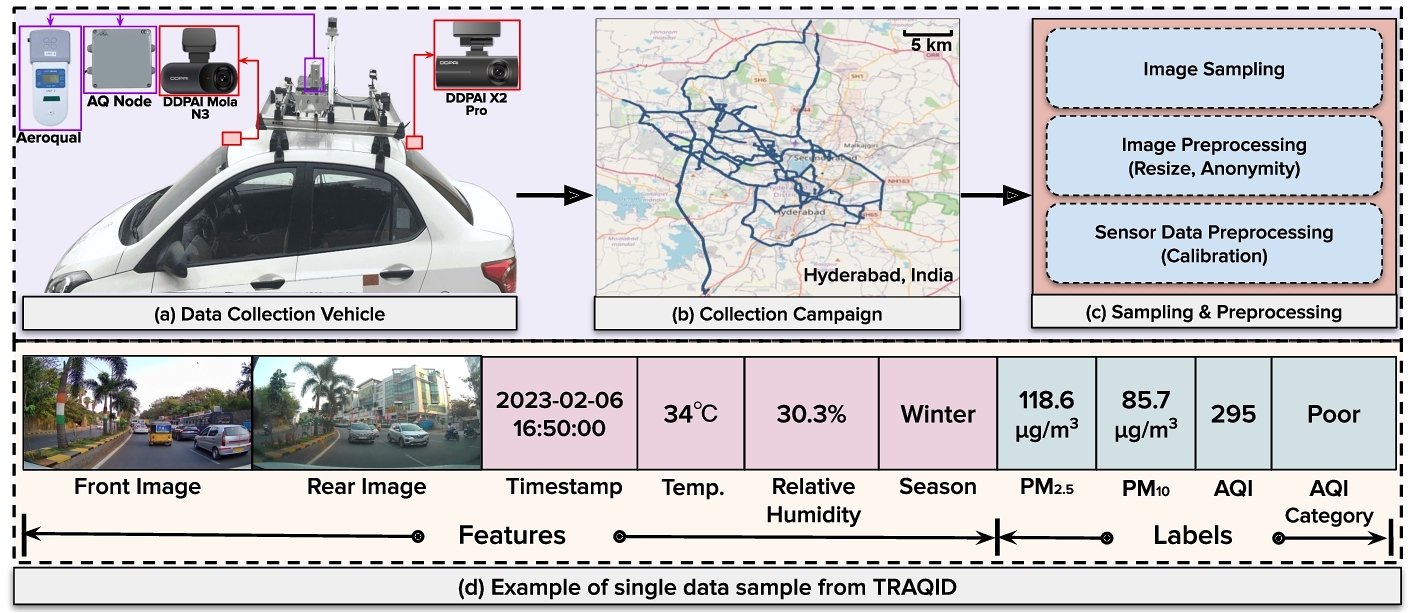
The data collection vehicle is equipped with two dashboard cameras as shown in Figure 2(a): 1. DDPAI Mola N3 [6] employed for front image capture, features a 5 MP CMOS sensor capable of recording in 2688 × 1944 ultra HD resolution, and 2. DDPAI X2 Pro [7] utilized for rear image capture, offers a 120° lens at the rear, ensuring a broad field of view while recording at 1920 × 1080 resolution. Both cameras record at a frame rate of 30 fps. These features facilitate high-quality image acquisition, enhancing data accuracy in urban settings.
The AQ Node is a custom device that measures PM concentrations and weather parameters at a frequency of 5 seconds. It includes an EspressIF ESP32 microcontroller unit (MCU) [33], a Nova SDS011 PM sensor [34] to measure PM2.5 and PM10 concentrations, and a BME280 sensor [11] to measure temperature and relative humidity. Additionally, an Aeroqual S500 [18], a reference device with a primary function of calibrating the PM sensors, was deployed, which captures a data point at a 1-minute frequency. The Nova PM sensor can measure particle size from 0.3 to 10 μm with a measuring range of 0.0 to 999.9 μg/m3. The AQ Node operates at a temperature range from -40°C to +125°C and a humidity range from 0% to 100% [28]. This equipment was mounted on the data collection vehicle to collect air quality data, capturing not only PM values but also the temperature and relative humidity, which are essential for assessing overall air quality [30].
2.2 Dataset Collection Campaign
The data collection campaign was conducted in the twin cities of Hyderabad and Secunderabad from October 2022 to July 2024, using the data collection vehicle shown in Figure 2(a). This vehicle travelled around the urban agglomeration, covering almost 2000 km at an average speed of 35 km/hr. The dataset collected in this campaign includes images extracted from 70+ hours of video, recorded on 20 distinct days across 6 different months in 3 years, ensuring diverse representation of environmental and traffic conditions in the twin cities. The specific route taken is detailed in Figure 2(b), with the paths plotted on OpenStreetMap [26] using GPS coordinates obtained from a mobile phone during the collection. The primary focus remained on collecting data within the city, with careful route planning to keep the vehicle within city limits. Samples were systematically collected throughout three distinct seasons: 1. Monsoon (October 2022, July 2024) 2. Winter (January, February and December 2023) and 3. Summer (March 2024) showcasing diverse climatic conditions.
Significance of City-Wide Coverage: The TRAQID dataset represents a significant advancement in air quality monitoring by providing comprehensive coverage of the twin cities of Hyderabad and Secunderabad. Capturing data across an entire urban agglomeration is a formidable task with several advantages. Firstly, it ensures the representation of diverse micro-environments within the cities, including residential areas, commercial zones, industrial sectors, and varying traffic densities. This diversity is crucial for developing robust air quality estimation models that can generalize across different urban settings. Secondly, the city-wide approach allows for capturing spatial variations in air quality, which can be significant even within short distances in urban areas due to localized pollution sources and varying topography. Moreover, the comprehensive nature of TRAQID facilitates the study of domain adaptation techniques for intercity air quality modelling. By capturing the full spectrum of urban environments, TRAQID provides a rich foundation for developing models that can potentially adapt to other urban areas, paving the way for more generalized air quality estimation systems across diverse city landscapes.
2.3 Image and Sensor Data Preprocessing
Image Data Preprocessing: The cameras mounted on the vehicle recorded 1-minute videos at a resolution of 1920 × 1080 and a frame rate of 30 fps. To align with the sampling rate of the sensors, we sampled images from the videos every 5 seconds to eliminate any repetitive frames and ensure consistency between the images and corresponding sensor data. Further, we filtered out outlier images manually, such as those affected by high amounts of headlight glare and extremely low illumination. The images were resized to 640 × 360 dimensions, making them compatible with deep learning architectures. To maintain dataset anonymity, we blurred both the number plates and faces within the images. Green-coloured number plates (indicating electric vehicles) were blurred while preserving their colour.
Sensor Data Preprocessing: To ensure the reliability of our air quality measurements, we implemented a rigorous calibration process for our low-cost PM sensors, following the method described by Ayu et al.[28]. This process involved comparing sensor readings against a reference device (Aeroqual S500) in a controlled environment, applying linear regression for calibration, and using the interquartile range (IQR) method to eliminate outliers. The resulting calibrated sensor data was then synchronized with our image captures, creating what we term “co-located” data points. This co-location approach is crucial for our vision-based air quality estimation task, as it establishes a direct temporal and spatial correspondence between the visual characteristics of traffic scenes and their associated air quality measurements. By ensuring this tight coupling between visual data and air quality parameters, we provide a solid foundation for developing and evaluating computer vision algorithms that can infer air quality from image content.
2.4 Dataset Description and Statistical Analysis
The proposed dataset contains a comprehensive compilation of 26,678 data samples, precisely gathered to ensure diversity across various environmental contexts. The dataset contains 13789 images obtained during the daytime (6 AM - 6 PM) and 12889 images obtained at nighttime (6 PM - 6 AM), which enables the possibility of predicting the AQI at different times of the day. This is especially useful for studying pollutants primarily observed at a particular time, such as smog, usually observed at night. The AQI values of the data samples are computed using the pollutants PM2.5 and PM10 concentration values as defined by the CPCB, India. Further, the AQI levels are categorized into six distinct classes which are as follows: 1. Good (0 - 50) 2. Satisfactory (51 - 100) 3. Moderate (101 - 200) 4. Poor (201 - 300) 5. Very Poor (301 - 400), and 6. Severe (> 400). As shown in Figure 2(d), each data sample comprises: 1. Front and rear images 2. Temperature (°C) 3. Relative humidity (%) 4. Season 5. Timestamp 6. PM2.5 concentration value 7. PM10 concentration value 8. AQI Value 9. AQI category (according to the CPCB standards). The front and rear images, with 640 × 360 × 3 dimensions, help understand the traffic scenario's vehicular dynamics. Temperature and relative humidity are scalar, and the season is categorical (summer, winter, monsoon). The timestamp contains the date and time of the sample captured. Another notable feature of the dataset is the sequential organization of the samples. Since the data was collected on 20 different dates, the data samples collected each day form a sequence, representing the progression of air quality as the data collection vehicle traverses the streets. For detailed dataset directory structure, refer to the supplementary material.
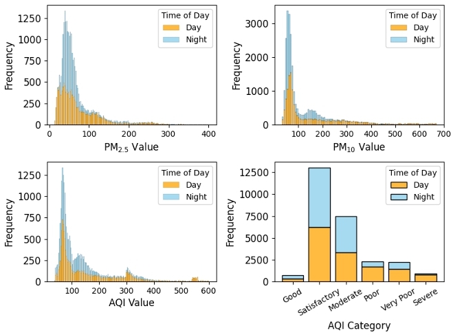
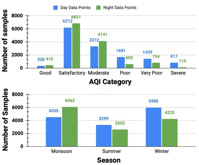
Figure 3 presents the histogram of labels for both day and night data samples. Figure 4 displays the dataset distribution across AQI categories and seasons, highlighting a deficiency in the “good” category compared to other categories. This suggests that AQI is generally adverse in traffic scenarios, with most data samples ranging from “satisfactory” to “moderate”, reflecting the typical air quality in Hyderabad city. The “poor”, “very poor”, and “severe” categories are significant, pointing to local events like construction activities, industrial operations, and open burning as contributing factors.
Analysis of air quality data reveals distinct seasonal and diurnal variations in pollutant concentrations and AQI categories. As shown in Table 2, monsoon season exhibited the best air quality with 643 ‘Good’ and 7,296 ‘Satisfactory’ AQI days, and the lowest mean AQI of 109. Conversely, summer presented the worst conditions, with zero ‘Good’ AQI days, the highest mean PM10 (209 μg/m3), and highest mean AQI (190). Winter recorded 601 ‘Severe’ AQI days and the highest mean PM2.5 (74 μg/m3). Diurnal patterns showed poorer daytime air quality (mean AQI 164) compared to nighttime (mean AQI 121), with higher frequencies of ‘Poor’, ‘Very Poor’, and ‘Severe’ categories during the day. PM10 levels consistently exceeded PM2.5 across all temporal divisions. Summer recorded the highest mean temperature (36° C) and lowest humidity (23%), while monsoon showed moderate temperatures (29° C) and high humidity (49%). These findings highlight the complex relationship between meteorological factors and air quality.
|
Good | Satisfactory | Moderate | Poor | Very Poor | Severe |
|
|
|
|
|
|
||||||||||||||
|---|---|---|---|---|---|---|---|---|---|---|---|---|---|---|---|---|---|---|---|---|---|---|---|---|---|---|
| Monsoon | 643 | 7296 | 1262 | 407 | 877 | 82 | 29 | 49 | 56 | 74 | 109 | 86 | ||||||||||||||
| Winter | 101 | 5656 | 1971 | 999 | 882 | 601 | 30 | 36 | 74 | 132 | 152 | 126 | ||||||||||||||
| Summer | 0 | 81 | 4220 | 877 | 474 | 249 | 36 | 23 | 73 | 209 | 190 | 90 | ||||||||||||||
| Day | 328 | 6212 | 3312 | 1681 | 1439 | 817 | 32 | 37 | 72 | 157 | 164 | 126 | ||||||||||||||
| Night | 416 | 6821 | 4141 | 602 | 794 | 115 | 29 | 39 | 60 | 92 | 121 | 80 |
3 Tasks
The primary objective behind the proposed dataset revolves around predicting air quality using both images and weather parameters. In the context of supervised learning, we define xi as single data point features which contains: images (front and rear), temperature, relative humidity, season, and timestamp. Conversely, yi denotes the corresponding ground truth labels, encompassing PM2.5, PM10, AQI value, and AQI category. Next, we outline the specific downstream tasks associated with this dataset.
Task 1: PM2.5 Estimation: Given a single data point xi, the objective is to estimate the PM2.5 concentration value as a real number.
Task 2: PM10 Estimation: Given a single data point xi, the objective is to estimate the PM10 concentration value as a real number.
Task 3: AQI Value Estimation: Given a single data point xi, the objective is to estimate the AQI value as a real number.
Task 4: AQI Category Estimation: Given a single data point xi, the objective is to classify the AQI into six distinct categories.
The initial three tasks are framed as regression challenges, whereas the final task is delineated as a classification problem. Addressing the classification task holds greater significance from an interpretability standpoint, as AQI categories offer more practical relevance in downstream applications. Furthermore, the sequential organization described in section 2 facilitates the establishment of connections between these data samples as a sequence. This adds valuable context and allows for the exploration of spatial patterns. By organizing the data as a sequence, advanced sequence modelling architectures can be used to capture and analyze the spatial dependencies present in the dataset.
4 Experiments and Benchmark Results
Drawing from the methodologies outlined in Section 1.2, we conducted benchmarking of the most effective approaches on the TRAQID dataset for the tasks specified in Section 3. The methods considered for benchmarking the dataset were those by Mondal et al.[22], Zhang et al.[38], Nilesh et al.[25], and Kalajdjieski et al.[15]. We split the TRAQID dataset into train 80%, validation 10% and test 10% sets. In regression tasks i.e. PM2.5 estimation, PM10 estimation, and AQI value estimation, performance evaluation was conducted using Root Mean Square Error (RMSE) and Mean Absolute Error (MAE) metrics. For the classification task, which is AQI category estimation, accuracy and F1-score metrics were used as performance evaluation. The hyperparameters are taken from the corresponding methodologies.
4.1 Experiments
As mentioned above, the following experiments were conducted to benchmark the specified methodologies on the TRAQID dataset. As defined in Mondal et al.[22], a modified version of the standard CNN framework was used to estimate PM2.5, PM10, AQI value and AQI categories. This architecture consisted of a total of 19 layers, encompassing both convolutional and fully connected layers, with approximately 4.8 million parameters in total. Rectified Linear Unit (ReLU) activation function was used, and the model was trained for 100 epochs with early stopping criteria and a learning rate of 1e− 3.
According to Zhang et al.[38], the AQC-Net was employed for both regression and classification tasks. The architecture contains a total of 0.03 million parameters. Training was conducted for 100 epochs with an initial learning rate of 1e− 2, subsequently reduced by a factor of 0.1 every 30 epochs.
As mentioned in Nilesh et al.[25], YOLOv5 was used to obtain vehicle counts from both rear and front images, which were subsequently aggregated to form the image features, while the weather features remained unchanged. However, since our dataset includes night images, the BRISQUE methodology was ineffective in determining image visibility scores and was excluded. For regression, RF regressor models predicted PM concentrations and AQI values, while RF classification models predicted AQI categories.
As defined in Kalajdjieski et al.[15], a multimodal architecture was implemented that leverages InceptionV3 [35] to extract image features, while a three-layer MLP with 64 neurons in each layer is utilized to extract weather features (including temperature, relative humidity, season, and timestamp categorized as day/night). The output feature vector from the MLP is concatenated with the output from InceptionV3 at the fully connected layer, which is then fed into a softmax layer for AQI category prediction. For regression tasks, instead of a softmax layer, a single neuron output layer is trained to predict PM or AQI values. The model contains approximately 24 million parameters. The model was trained for 100 epochs with a learning rate of 1e− 3, using the early stopping criteria.
| Method |
|
|
|
|
||||||||
|---|---|---|---|---|---|---|---|---|---|---|---|---|
| RMSE ↓ | MAE ↓ | RMSE ↓ | MAE ↓ | RMSE ↓ | MAE ↓ | Accuracy ↑ | F1-Score ↑ | |||||
| Mondal et al.[22] | 32.81 | 19.50 | 55.65 | 30.62 | 60.34 | 36.69 | 0.64 | 0.61 | ||||
| Kalajdjieski et al.[15] | 33.90 | 21.47 | 51.47 | 27.39 | 68.28 | 41.07 | 0.60 | 0.56 | ||||
| Nilesh et al.[25] | 22.62 | 13.68 | 46.25 | 22.57 | 54.24 | 33.19 | 0.73 | 0.71 | ||||
| AQC-Net [38] | 23.31 | 14.45 | 44.23 | 21.23 | 52.21 | 31.67 | 0.75 | 0.74 | ||||
For all the methodologies implemented above, the Mean Squared Error (MSE) loss function was used for regression tasks, while the cross-entropy loss function was utilized for classification tasks. In [15, 22, 38], the TRAQID dataset's front and rear images were sequentially processed by their respective CNN model. Subsequently, the outputs were concatenated and passed to the fully connected layer. PyTorch [29] was utilized for all implementations.
4.2 Results
The results of the methodologies on the TRAQID dataset are presented in Table 3. It is clearly observed that the conventional CNN models used by [15, 22] fail to grasp the intricacies of the task at hand. This is primarily due to the fact that standard CNN models may struggle to incorporate the diverse factors affecting air quality, including industrial activities, construction, environmental variations, and geographical features, into their predictions. AQC-Net [38] stands out among the methods, demonstrating superior performance in three tasks which is PM10 estimation, AQI value estimation and AQI category estimation. This highlights the effectiveness of attention-based methods in identifying pollution-contributing objects in images. However, the top F1-score achieved for the AQI category estimation task is just 0.74, highlighting the significant impact of dataset size and diversity on the complexity of the task. Inclusion of nighttime images brings challenges like low illumination and glare through headlights which makes the task at hand more complicated in compare to the datasets which only contains daytime images.
| Season/Time |
|
|
|
|
||||||||||||
|---|---|---|---|---|---|---|---|---|---|---|---|---|---|---|---|---|
| RMSE ↓ | MAE ↓ | RMSE ↓ | MAE ↓ | RMSE ↓ | MAE ↓ | Acc ↑ | F1-Score ↑ | |||||||||
| Monsoon | 19.70 | 10.16 | 14.91 | 8.56 | 37.57 | 20.86 | 0.78 | 0.76 | ||||||||
| Winter | 16.84 | 9.76 | 36.67 | 17.30 | 43.01 | 24.63 | 0.79 | 0.78 | ||||||||
| Summer | 29.12 | 16.66 | 72.78 | 48.08 | 69.80 | 46.03 | 0.73 | 0.68 | ||||||||
| Day | 25.73 | 14.37 | 54.93 | 28.17 | 59.40 | 34.54 | 0.76 | 0.74 | ||||||||
| Night | 17.25 | 9.14 | 26.59 | 12.68 | 37.71 | 21.21 | 0.80 | 0.79 | ||||||||
| Front | 29.32 | 18.78 | 52.53 | 28.76 | 60.39 | 41.45 | 0.72 | 0.70 | ||||||||
| Rear | 31.68 | 21.35 | 53.89 | 29.43 | 65.23 | 43.87 | 0.69 | 0.68 | ||||||||
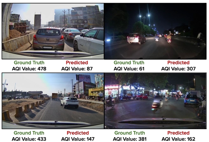
Nilesh et al.[25] achieved the highest score in PM2.5 estimation task, demonstrating that incorporating vehicle counts alongside weather parameters can aid in air quality estimation. This can be viewed as a specific instance of attention mechanism, where vehicle emissions constitute a significant pollution source on roads and streets. It suggests a positive correlation between traffic volume and pollution levels. However, the model achieved only a 0.71 F1-score for the AQI category estimation task, representing a 10% decrease for the same task compared to their proposed dataset. This reduction may be attributed to the improved season diversity in our dataset, feature not present in previous datasets. Additionally, the presence of unstructured traffic further complicates the task. Figure 5 shows some of the classification challenges associated with the dataset. The top and bottom left figures show data samples having high ground truth AQI value. However, the best-performing model for this task predicts a very low AQI value, indicating a failure to detect pollution caused by nearby bridge construction. Similarly, the model struggles with low illumination in the top right image and unstructured traffic scenario in the bottom right image. Please refer to the supplementary material for further insights into the dataset challenges.
4.3 Seasonal and Diurnal Variations
To investigate seasonal and diurnal variations, we segmented the dataset into multiple splits. For seasonal analysis, we created three subsets: 1. Monsoon, 2. Winter, and 3. Summer. For diurnal analysis, we divided the data into two categories: 1. Day and 2. Night. Each of these split datasets was further partitioned into training (80%) and validation (20%) sets. We then trained the best-performing model for all four defined tasks to each of these datasets. Table 4 presents the results for each dataset.
The challenge of modeling summer data is evident, even for the best-performing model, primarily due to the fluctuation in temperature and humidity during summers. Conversely, the model achieved its best performance on monsoon data, likely because a majority of the data samples fall within the 0 - 200 AQI range, attributed to the rainfall during the monsoon season. As for the day/night comparison, the model exhibited superior performance in predicting nighttime air quality parameters compared to daytime. This can be attributed to several factors: reduced human activity and more stable meteorological conditions at night, resulting in lower variability in air quality (as shown in Fig. 3 and Table 2); a more stable atmospheric boundary layer, leading to consistent pollutant concentrations; and fewer extreme AQI categories (“Poor”, “Very Poor”, “Severe”) at night, which aligns with the model's tendency to perform better on less extreme values. The reduced influence of rapid fluctuations from daytime events (e.g., rush hour traffic, sudden weather changes) likely enhances the model's nighttime predictions. Analysis of camera perspectives revealed inferior performance when using single views, with front-view models performing marginally better than rear-view models. This indicates the importance of utilizing both camera perspectives for optimal air quality prediction.
4.4 Interpreting AQI Predictions via GradCAM
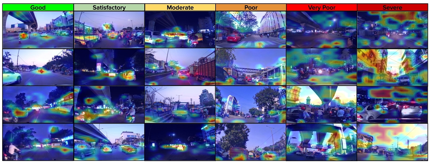
To visualize and interpret the AQC-Net [38] decision-making process for AQI category estimation, we employed Gradient-weighted Class Activation Mapping (GradCAM) [31]. The GradCAM technique was applied to the final convolutional layer of the trained model, generating heatmaps that highlight the regions of input images most influential in determining the predicted AQI category. These visualizations were generated for multiple images across different AQI categories to analyze how the model's focus shifts with varying air quality conditions. As illustrated in Fig. 6, the model consistently focuses on vehicles, particularly their exhaust areas, across all AQI categories, indicating its recognition of vehicular emissions as a crucial air quality factor. For “Good”, “Satisfactory”, and “Moderate” categories, the model attends to urban structures such as flyovers, buildings, and bridges. However, as AQI deteriorates from “Poor” to “Severe”, attention shifts towards open areas and light sources, potentially seeking indicators of haze or atmospheric clarity. Notably, in “Severe” AQI images, the model considers broader image portions, suggesting an analysis of overall atmospheric conditions rather than specific pollution sources. These observations suggest that the model has learned to associate air quality with complex set of visual cues related to traffic patterns, urban infrastructure, and atmospheric conditions.
5 Conclusion and Future Work
This paper introduced TRAQID, a novel dataset capturing 26,678 images of traffic across Hyderabad and Secunderabad, India, alongside co-located air quality parameters (PM2.5, PM10, AQI value, and AQI category) and weather data (temperature and humidity). The dataset's uniqueness lies in its front and rear camera setup, capturing both day and night environments across different seasons. It has a sequential arrangement of co-located data samples representing the mobile traffic capture. By applying state-of-the-art image-based algorithms on this dataset for estimating PM2.5, PM10, AQI value, and category, we demonstrated that existing algorithms struggle with such a diverse dataset spanning various seasons and times of day. This underscores the importance of TRAQID in developing robust methodologies for air quality classification and prediction. Our GradCAM analysis revealed that the best-performing model, AQC-Net, focuses on vehicles, urban structures, and atmospheric conditions across different AQI categories, providing insights into its decision-making process.
Future work based on TRAQID could include developing novel image-based AQI estimation methods specifically tailored for traffic conditions, leveraging the dataset's front and rear image features as well as the sequential arrangement of co-located data samples. Additionally, TRAQID can facilitate research on several downstream tasks, such as traffic density estimation, vehicle type classification, urban infrastructure analysis, and studying correlations between traffic patterns and air quality.
Acknowledgments
We thank iHubData, IIIT Hyderabad for extending research fellowship and Bodhyan platform support for curating the novel dataset.
References
- Maqsood Ahmed et al. 2022. AQE-Net: A deep learning model for estimating air quality of Karachi city from mobile images. Remote Sensing 14, 22 (2022), 5732.
- Thomas Becnel, Kyle Tingey, Jonathan Whitaker, Tofigh Sayahi, Katrina Lê, Pascal Goffin, Anthony Butterfield, Kerry Kelly, and Pierre-Emmanuel Gaillardon. 2019. A Distributed Low-Cost Pollution Monitoring Platform. IEEE Internet of Things Journal 6, 6 (2019), 10738–10748.
- Sean D. Beevers and Martin L. Williams. 2020. Chapter 6 - Traffic-related air pollution and exposure assessment. In Traffic-Related Air Pollution, Haneen Khreis, Mark Nieuwenhuijsen, Josias Zietsman, and Tara Ramani (Eds.). Elsevier, 137–162.
- Leo Breiman. 2001. Random forests. Machine learning 45 (2001), 5–32.
- Peter Carr and Richard Hartley. 2009. Improved single image dehazing using geometry. In Digital Image Computing: Techniques and Applications. IEEE, 103–110.
- DDPAI. 2022. DDPAI Mola N3 Dash Camera. https://en.ddpai.com/products/molan3dashcam.html. [Accessed 07-08-2024].
- DDPAI. 2022. DDPAI X2 Pro Dash Camera. https://en.ddpai.com/products/x2sprodashcam.html. [Accessed 07-08-2024].
- Glenn Jocher et. al.2022. ultralytics/yolov5: v7.0 - YOLOv5 SOTA Realtime Instance Segmentation. https://doi.org/10.5281/zenodo.7347926.
- Raanan Fattal. 2008. Single image dehazing. ACM transactions on graphics (TOG) 27, 3 (2008), 1–9.
- Raanan Fattal. 2014. Dehazing using color-lines. ACM transactions on graphics (TOG) 34, 1 (2014), 1–14.
- Bosch Sensortec GmbH. 2015. Bosch BME 280. https://www.bosch-sensortec.com/products/environmental-sensors/humidity-sensors-bme280/. [Accessed 07-08-2024].
- Government of Telangana. 2024. Telangana Transport Department. https://www.transport.telangana.gov.in/html/statistics_vehicles.html. [Accessed 07-08-2024].
- Kaiming He, Xiangyu Zhang, Shaoqing Ren, and Jian Sun. 2016. Deep residual learning for image recognition. In Proceedings of the IEEE conference on computer vision and pattern recognition. 770–778.
- Central Pollution Control Board India. 2015. Report on AQI Control of Urban Pollution Series. http://app.cpcbccr.com/ccr_docs/FINAL-REPORT_AQI_.pdf. [Accessed 07-08-2024].
- Jovan Kalajdjieski, Eftim Zdravevski, Roberto Corizzo, Petre Lameski, Slobodan Kalajdziski, Ivan Miguel Pires, Nuno M Garcia, and Vladimir Trajkovik. 2020. Air pollution prediction with multi-modal data and deep neural networks. Remote Sensing 12, 24 (2020), 4142.
- G Kaushik, A Chel, S Patil, and S Chaturvedi. 2019. Status of particulate matter pollution in India: a review. Handbook of Environmental Materials Management (2019), 167–193.
- Pu-Yun Kow, I-Wen Hsia, Li-Chiu Chang, and Fi-John Chang. 2022. Real-time image-based air quality estimation by deep learning neural networks. Journal of Environmental Management 307 (2022), 114560.
- Aeroqual Limited. 2021. Aeroqual S500. https://www.aeroqual.com/products/s-series-portable-air-monitors/series-500-portable-indoor-monitor. [Accessed 07-08-2024].
- Chenbin Liu, Francis Tsow, Yi Zou, and Nongjian Tao. 2016. Particle pollution estimation based on image analysis. PloS one 11, 2 (2016).
- Earl J McCartney. 1976. Optics of the atmosphere: scattering by molecules and particles. New York (1976).
- Anish Mittal, Anush Krishna Moorthy, and Alan Conrad Bovik. 2012. No-Reference Image Quality Assessment in the Spatial Domain. IEEE Transactions on Image Processing 21, 12 (2012), 4695–4708.
- Joyanta Jyoti Mondal, Md Farhadul Islam, Raima Islam, Nowsin Kabir Rhidi, Sarfaraz Newaz, Meem Arafat Manab, ABM Alim Al Islam, and Jannatun Noor. 2024. Uncovering local aggregated air quality index with smartphone captured images leveraging efficient deep convolutional neural network. Scientific Reports 14, 1 (2024), 1627.
- Srinivasa G Narasimhan and Shree K Nayar. 2002. Vision and the atmosphere. International journal of computer vision 48 (2002), 233–254.
- IBM Newsroom. 2015. IBM Expands Green Horizons Initiative Globally To Address Pressing Environmental and Pollution Challenges. https://uk.newsroom.ibm.com/2015-Dec-09-IBM-Expands-Green-Horizons-Initiative-Globally-To-Address-Pressing-Environmental-and-Pollution-Challenges. [Accessed 07-08-2024].
- Nitin Nilesh, Ishan Patwardhan, Jayati Narang, and Sachin Chaudhari. 2022. IoT-based AQI estimation using image processing and learning methods. In 2022 IEEE 8th World Forum on Internet of Things (WF-IoT). IEEE, 1–5.
- OpenStreetMap contributors. 2017. Planet dump retrieved from https://planet.osm.org. https://www.openstreetmap.org. [Accessed 07-08-2024].
- Google Earth Outreach. 2017. Air Quality. https://www.google.com/earth/outreach/special-projects/air-quality/. [Accessed 07-08-2024].
- Ayu Parmar, Spanddhana Sara, Ayush Kumar Dwivedi, C Rajashekar Reddy, Ishan Patwardhan, Sai Dinesh Bijjam, Sachin Chaudhari, KS Rajan, and Kavita Vemuri. 2024. Development of end-to-end low-cost IoT system for densely deployed PM monitoring network: an Indian case study. Frontiers in The Internet of Things 3 (2024), 1332322.
- Adam Paszke et al. 2019. Pytorch: An imperative style, high-performance deep learning library. Advances in neural information processing systems 32 (2019).
- Vaishali Sagar, Gaurav Verma, and Rupesh Das. 2023. Influence of Temperature and Relative Humidity on PM2.5 Concentration over Delhi. Mapan - Journal of Metrology Society of India 38 (05 2023).
- Ramprasaath R. Selvaraju, Michael Cogswell, Abhishek Das, Ramakrishna Vedantam, Devi Parikh, and Dhruv Batra. 2017. Grad-CAM: Visual Explanations from Deep Networks via Gradient-Based Localization. In 2017 IEEE International Conference on Computer Vision (ICCV). 618–626.
- Geoff Spencer. 2018. AI for Earth: Helping save the planet with data science. https://news.microsoft.com/apac/features/ai-for-earth-helping-save-the-planet-with-data-science/. [Accessed 07-08-2024].
- Espressif Systems. 2022. ESPRESSIF ESP 32. https://www.espressif.com/en/products/socs/esp32. [Accessed 07-08-2024].
- Nova Analytical Systems. 2022. NOVA Air Quality Sensor SDS011. https://www.nova-gas.com/. [Accessed 07-08-2024].
- Christian Szegedy, Vincent Vanhoucke, Sergey Ioffe, Jon Shlens, and Zbigniew Wojna. 2016. Rethinking the Inception Architecture for Computer Vision. In Proceedings of the IEEE Conference on Computer Vision and Pattern Recognition (CVPR).
- WHO. 2024. WHO(World Health Organisation). https://www.who.int/health-topics/air-pollution. [Accessed 07-08-2024].
- Kai Zhang and Stuart Batterman. 2013. Air pollution and health risks due to vehicle traffic. Science of the total Environment 450 (2013), 307–316.
- Qiang Zhang, Fengchen Fu, and Ran Tian. 2020. A deep learning and image-based model for air quality estimation. Science of The Total Environment 724 (2020), 138178.
Footnote
1 https://airquality.cpcb.gov.in/AQI_India/

This work is licensed under a Creative Commons Attribution International 4.0 License.
ICVGIP 2024, December 13–15, 2024, Bengaluru, India
© 2024 Copyright held by the owner/author(s).
ACM ISBN 979-8-4007-1075-9/24/12.
DOI: https://doi.org/10.1145/3702250.3702260