FROST: Foundation-model Representations with Domain Knowledge for Spatially and Temporally Robust Frost Prediction
DOI: https://doi.org/10.1145/3765611.3815487
ACM Sustainability Week Companion '26: ACM Sustainability Week 2026, Banff, AB, Canada, June 2026
Frost is a major agricultural hazard driven by localized microclimate conditions, making accurate and transferable prediction challenging. Existing approaches either rely on hand-crafted domain-knowledge based features with classical models, which offer spatial robustness but limited temporal modeling, or deep sequence models, which capture short-term dynamics but overfit to location-specific patterns and fail to generalize. We address these limitations with a hybrid framework that achieves both spatial and temporal robustness by combining domain knowledge with representations from a time series foundation model (TSFM). Specifically, we deploy a pre-trained TSFM in a zero-shot manner to extract station-agnostic temporal features, avoiding fine-tuning to preserve generalization. We then integrate a compressed TSFM embedding and its direct temperature forecast with hand-crafted meteorological features, and train a lightweight predictor for efficient deployment. Experiments on multi-year California weather station data under both temporal and spatial test settings show that our approach consistently outperforms classical and deep sequential baselines, achieving superior accuracy and calibration, particularly at longer prediction horizons. These results demonstrate that zero-shot TSFM representations, when combined with domain features, provide a practical and spatially and temporally robust solution for frost prediction.
ACM Reference Format:
Hui Wei, Dong Yoon Lee, and Shijia Pan. 2026. FROST: Foundation-model Representations with Domain Knowledge for Spatially and Temporally Robust Frost Prediction. In ACM Sustainability Week 2026 (ACM Sustainability Week Companion '26), June 22--25, 2026, Banff, AB, Canada. ACM, New York, NY, USA 5 Pages. https://doi.org/10.1145/3765611.3815487
1 Introduction
Frost occurs when near-surface air temperatures fall below freezing, forming ice crystals that can damage or destroy plant tissue within hours. It is one of the most economically significant meteorological hazards in agriculture, causing billions of dollars in annual crop losses worldwide [4, 14, 16]. Early and reliable prediction is critical, as sufficient lead time enables farmers to deploy protective measures (e.g., heaters or wind machines), ultimately determining whether crops are saved or lost. However, accurate prediction remains challenging due to the complex, multiscale processes governing frost formation [19]. Moreover, frost is a microclimate phenomenon influenced by local topography, elevation, and land cover, making coarse regional forecasts (e.g., HRRR1, NWP2) insufficient for accurate local frost prediction [20].
Recent studies have explored the use of meteorological data collected from local weather stations, combined with machine learning (ML) approaches capable of learning complex patterns for frost prediction. Current approaches fall into two categories: classical machine learning models (e.g., linear regression, random forests) trained on hand-crafted meteorological features (e.g., dew point depression, cooling rate) [3, 5, 7, 8, 10, 15, 17, 18], and deep sequence models (e.g., GRU [6], TCN [1]) trained end-to-end on raw meteorological time series [2, 21]. These two types of approaches have different strengths. Deep sequence models are well-suited to short-term prediction: weather conditions are highly persistent over a few hours, so recent measurements of temperature, humidity, and wind reliably predict the near future, patterns that sequence models capture effectively. However, because they train on location-specific data, they inevitably encode local climate patterns that do not transfer well to new sites. Classical ML models instead use features based on universal physical understanding of frost formation (e.g., dew-point depression, cooling rate) that apply across locations, giving them greater spatial robustness. They also remain informative at longer horizons, where recent observations become less predictive and frost risk depends more on physical preconditions (e.g., humidity, wind calm) that hand-crafted features directly encode.
This paper aims to achieve two goals: (G1) Spatial robustness. Because frost is a microclimate phenomenon, risk varies sharply with local topography, elevation, and land cover, factors that differ even between nearby stations. Models must generalize to previously unmonitored (out-of-network) stations to be practically deployable across diverse agricultural settings; and (G2) Temporal robustness. Longer prediction horizons give farmers more lead time to deploy protective measures. Models must maintain reliable performance across horizons, from short-term (3 h) to day-ahead (24 h) predictions. Motivated by the distinct strengths of these two types, we propose a hybrid approach that integrates their strengths to achieve spatial (G1) and temporal (G2) robustness. Rather than training a deep sequence model from scratch on location-specific data, which embeds station-specific patterns that limit transfer to new sites, we use a time series foundation model (TSFM) [12] as the temporal encoder in a zero-shot manner. Pre-trained on large-scale, diverse data, a TSFM retains the temporal modeling capabilities of deep sequence models while producing more general, station-agnostic representations; fine-tuning would reintroduce station-specific microclimate patterns and is therefore avoided. However, a central challenge in this hybrid design is that TSFM representations and hand-crafted features reside in different feature spaces: TSFM outputs are high-dimensional vectors encoding complex temporal dynamics, while hand-crafted features are compact scalars grounded in domain physics.
To bridge this gap, we project the TSFM's output representation, which encodes the full temporal context window in a compact vector, into a lower-dimensional space. We additionally include the TSFM's direct prediction of minimum air temperature alongside the reduced representation – this forecast provides an explicit, task-relevant signal directly tied to frost risk. Both TSFM-derived features, combined with hand-crafted domain features, are then passed to a prediction head to achieve improved spatial and horizon robustness.
Experiments on a multi-year dataset of California agricultural weather stations evaluate our system against six baselines under temporal and spatial evaluation protocols at four prediction horizons (3, 6, 12, and 24 h). Our model achieves the best frost detection accuracy (AUPRC) and calibration (Brier score) at ≥ 6 h on both holdouts. Crucially, while purely temporal baselines degrade substantially when transferred to unseen out-of-network stations, our hybrid system generalizes more robustly under distribution shift.
2 Methodology
We focus on improving spatial and temporal robustness in frost prediction task, which is formulated as two coupled tasks: regression to predict the minimum air temperature ($T_\text{min}$) and classification to identify frost events. We address these robustness challenges through two components: (1) a hybrid architecture that combines both the domain knowledge for long-term forecasting and the station-agnostic generalizability of foundational model. (2) strategies to address data imbalance of rare frost events.
Task Description. Given multivariate meteorological observations over [t − Tc, t − 1], we predict conditions over [t, t + Tp − 1]; the regression output quantifies frost severity to calibrate protective intervention efforts (e.g., heater temperature), while the classification determines whether to act.
In order to reflect the biological reality that plant tissue damage progresses gradually near the frost boundary and accounts for sensor uncertainty at the critical threshold, we map the predicted temperature to a frost probability via the logistic function $P = [1 + \exp (2(T_\text{pred} - T_\text{threshold}))]^{-1}$, rather than applying a hard threshold to get the binary class (frost vs. non-frost). We use commonly used $T_\text{threshold} = 0^\circ \text{C}$ in this work, though the framework also supports species-specific thresholds (e.g., − 2.2°C for blossoming almonds).
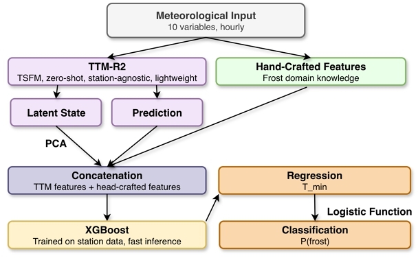
Hybrid Architecture. We propose a hybrid architecture leveraging both generalizable temporal representations and domain-specific physical knowledge in hand-crafted features to achieve spatial and horizon robustness. Figure 1 provides the model overview.
Our design prioritizes spatial generalization and deployability under resource constraints. To avoid encoding station-specific patterns that may harm transfer to unseen locations, we adopt a zero-shot temporal encoder with fixed representations. Concretely, we use TinyTimeMixer (TTM-R2) [9], a lightweight multivariate MLP-Mixer–based TSFM (1M parameters, 3.4 MB), well-suited to CPU-only deployments at previously unmonitored agricultural sites. TTM processes a fixed 512-hour context window of raw meteorological time series, and we keep its weights frozen during training.
Additionally, we aim to capture both an explicit forecast signal and a rich representation of current thermal dynamics, as these complementary cues improve downstream prediction. Accordingly, from a single TTM forward pass, we extract two components. First, we use TTM's 96-step forecast and take the minimum over horizon h, $\hat{y}_\text{TTM} = \min (\mathbf {p}_{1:h})$, as a globally contextualized estimate of $T_\text{min}$ based on the 512-hour history. Second, we extract the 128-dimensional hidden-state embedding from the most recent temporal patch of the final encoder layer. This patch emphasizes the current thermal state most relevant to imminent frost while still incorporating prior context through cross-patch mixing, consistent with the atmospheric persistence signal observed in our ablations. Together, the scalar forecast and embedding are complementary: the former provides an explicit prediction, while the latter captures latent structure not reflected in the scalar output.
To balance representational efficiency and preserve the influence of domain features, we compress the TTM embedding before passing it to the prediction head. Specifically, we apply PCA to reduce its dimensionality from 128 to 16. This removes redundant, highly correlated directions while retaining the dominant modes of thermal variability, and prevents the embedding from overwhelming the feature space due to its otherwise much higher dimensionality compared to the hand-crafted and scalar features.
In order to ensure efficient and robust prediction under resource-constrained, real-world deployments, we adopt a lightweight model that supports fast CPU inference and handles missing data natively. Accordingly, we concatenate the hand-crafted features (Section 3), TTM PCA components, and the TTM scalar prediction into a single feature vector and feed it to an XGBoost regressor [5]. Its sequential boosting yields compact models with low memory overhead, avoiding the need to store and evaluate many independent trees as in bagging-based methods like Random Forest. In addition, XGBoost's native handling of missing values is critical during the cold-start phase at newly deployed stations, where the full 512-hour TTM context window may be unavailable, eliminating the need for explicit imputation.
Strategies to Address Data Imbalance. Frost events are rare relative to non-frost conditions (account for less than 1% in our dataset), so a standard MSE objective would bias the model toward warm-weather accuracy and under-predict frost severity. To address this imbalance, we adopt a two-level weighting strategy that emphasizes both rare samples and difficult predictions.
At the sample level, each instance is assigned a weight w(y) based on its ground-truth minimum temperature y. Frost samples (y ≤ 0) receive the maximum weight $w_\text{max}$, while non-frost weights decay exponentially toward $w_\text{min}=1$ as temperature increases, so that values above + 5°C receive minimal upweighting:
(1)
Rather than treating frost prevalence as a fixed hyperparameter, $w_\text{max}$ is set adaptively as the inverse of the training frost rate $p_\text{frost}$, capped at 50 to prevent gradient instability:
(2)
This adaptive design ensures the weighting scales automatically with frost rarity across training splits, making it robust to temporal variation in frost frequency.
At the loss level, we further emphasize hard examples using a focal-style regression objective inspired by Lin et al. [13]. Specifically, we generalize the quadratic loss by raising the absolute error to the power 2 + γ :
(3)
3 Experiments
Data. Experiments are conducted on data from 29 CIMIS3 meteorological stations across California's Central Valley, one of the most productive agricultural regions in the world. Twenty stations provide hourly records from 2010–2025 (in-network); the remaining 9 provide data from 2023–2025 (out-of-network). Frost events ($T_\text{min} < 0^\circ \text{C}$) account for less than 1% of all instances, reflecting the severe class imbalance inherent to the domain.
Features. Each station records 10 hourly meteorological variables: air temperature, dew point, relative humidity, soil temperature, wind speed, wind direction, solar radiation, vapor pressure, precipitation, and evapotranspiration. From these, we construct 44 hand-crafted features in five groups: (1) temporal statistics: mean, min, and max over the 72h context window for each variable (30 features); (2) cyclic time encodings: sin/cos of hour-of-day and day-of-year (4 features); (3) static location: elevation, latitude, longitude (3 features); (4) previous-day mirror window: minimum air temperature and sub-zero duration over the preceding 24h (2 features); and (5) physical derived aggregates: dew point depression, soil–air temperature difference, and hourly cooling rate (5 features).
Train and Evaluation Protocol. 20 in-network stations are split temporally: 2010–2022 for training, 2022–2023 for validation, and 2023–2025 as the temporal test set. 9 out-of-network stations (2023–2025) serve as the spatial test set. All baselines and hand-crafted features use a 72-hour context window, capturing 3 complete diurnal cycles, the natural timescale of synoptic frost-driving weather systems. Empirically, extending this window beyond 72 hours yields negligible gains for all baselines. Our model further benefits from TTM's 512-hour receptive field, an inherent property of the pre-trained foundation model, enabling it to capture longer temporal context. We assess four prediction horizon (3, 6, 12, 24 h), training a separate model per horizon.
Baselines. We compare against seven baselines across three categories. Heuristic: previous-day same-period minimum temperature (Prev-Day). Classical ML (operating on hand-crafted features): Linear Regression (LR) [7, 15], MLP [8, 18], Random Forest [3, 7], and XGBoost [5, 10, 17]. Deep sequence models (operating on raw 72h multivariate time series): GRU [2, 6] and TCN [1, 2], each with an MLP prediction head and RevIN normalization [11] to mitigate distribution shift.
Evaluation Metrics. We report MAE for temperature regression. For frost classification, we report AUPRC and Brier score. AUPRC is preferred over AUROC under extreme class imbalance, and over threshold-dependent metrics (e.g., precision, recall) because the optimal decision threshold varies with the Cost-Loss ratio of each farming operation. Brier score measures probability calibration, directly reflecting the reliability of the prediction.
4 Results
Temporal and Spatial Testing Results. Table 1 reports MAE, AUPRC, and Brier score across all models and prediction horizons on both temporal and spatial test sets. Our hybrid model demonstrates consistent advantages on AUPRC and Brier score, the metrics most directly relevant to operational frost warning, while remaining competitive on MAE. On the temporal test set, our model leads all baselines on AUPRC from 6h onward with a margin that grows with prediction horizon, reaching +0.048 over the next-best model at 12h and +0.013 at 24h. The advantage becomes substantially larger on the spatial test set, where models must generalize to unmonitored stations with no training data. At 24h, GRU and TCN suffer a severe AUPRC collapse to 0.519 and 0.520 respectively, rendering them no better than the naive previous-day baseline (0.528), whereas our model retains 0.579, the only model to maintain a meaningful advantage. A parallel deterioration appears in Brier score: GRU and TCN degrade by 65% from temporal to spatial test set at 24h (0.017 → 0.028), while our model degrades by only 38% (0.016 → 0.022). We attribute this robustness to the hand-crafted geographic and physical features, elevation, latitude, dew point depression, and soil-air temperature difference, which encode universal thermodynamic and topographic signals that transfer directly to unseen stations, providing the stable inductive bias that purely data-driven temporal models lack. These results confirm that our hybrid architecture achieves both spatial robustness (G1) and temporal robustness (G2): it leads all baselines on AUPRC and Brier score from 6h through 24h, while maintaining accurate frost detection at unseen out-of-network stations where other baseline models usually fail.
| Horizon | Model | AUPRC (↑) | Brier (↓) | MAE (↓) | |||
|---|---|---|---|---|---|---|---|
| T | S | T | S | T | S | ||
| 3h | Prev-Day | 0.421 | 0.371 | 0.006 | 0.009 | 2.053 | 2.220 |
| LR | 0.393 | 0.515 | 0.009 | 0.010 | 2.196 | 2.323 | |
| MLP | 0.727 | 0.718 | 0.004 | 0.005 | 1.327 | 1.521 | |
| RF | 0.600 | 0.649 | 0.005 | 0.005 | 2.302 | 2.368 | |
| XGBoost | 0.723 | 0.719 | 0.004 | 0.005 | 1.315 | 1.480 | |
| GRU | 0.874 | 0.877 | 0.002 | 0.003 | 0.761 | 0.864 | |
| TCN | 0.847 | 0.879 | 0.002 | 0.003 | 0.855 | 0.982 | |
| Ours | 0.865 | 0.842 | 0.003 | 0.003 | 0.930 | 1.036 | |
| 6h | Prev-Day | 0.455 | 0.398 | 0.010 | 0.013 | 2.023 | 2.201 |
| LR | 0.467 | 0.529 | 0.012 | 0.014 | 2.236 | 2.364 | |
| MLP | 0.677 | 0.676 | 0.006 | 0.008 | 1.408 | 1.642 | |
| RF | 0.583 | 0.626 | 0.008 | 0.008 | 2.230 | 2.306 | |
| XGBoost | 0.684 | 0.668 | 0.006 | 0.008 | 1.437 | 1.618 | |
| GRU | 0.785 | 0.740 | 0.005 | 0.007 | 0.974 | 1.154 | |
| TCN | 0.791 | 0.790 | 0.005 | 0.006 | 1.087 | 1.279 | |
| Ours | 0.814 | 0.784 | 0.004 | 0.006 | 1.143 | 1.279 | |
| 12h | Prev-Day | 0.472 | 0.418 | 0.015 | 0.019 | 2.016 | 2.228 |
| LR | 0.533 | 0.546 | 0.015 | 0.017 | 1.992 | 2.116 | |
| MLP | 0.664 | 0.629 | 0.010 | 0.012 | 1.519 | 1.743 | |
| RF | 0.596 | 0.552 | 0.012 | 0.014 | 2.023 | 2.120 | |
| XGBoost | 0.672 | 0.597 | 0.010 | 0.013 | 1.557 | 1.738 | |
| GRU | 0.699 | 0.568 | 0.009 | 0.015 | 1.253 | 1.525 | |
| TCN | 0.707 | 0.678 | 0.009 | 0.012 | 1.317 | 1.538 | |
| Ours | 0.755 | 0.706 | 0.008 | 0.011 | 1.363 | 1.538 | |
| 24h | Prev-Day | 0.567 | 0.528 | 0.022 | 0.027 | 1.870 | 2.042 |
| LR | 0.599 | 0.500 | 0.020 | 0.026 | 1.804 | 2.001 | |
| MLP | 0.640 | 0.568 | 0.018 | 0.022 | 1.647 | 1.863 | |
| RF | 0.605 | 0.544 | 0.020 | 0.024 | 1.839 | 1.995 | |
| XGBoost | 0.641 | 0.516 | 0.018 | 0.024 | 1.672 | 1.855 | |
| GRU | 0.682 | 0.519 | 0.017 | 0.028 | 1.486 | 1.787 | |
| TCN | 0.688 | 0.520 | 0.017 | 0.028 | 1.501 | 1.780 | |
| Ours | 0.701 | 0.579 | 0.016 | 0.022 | 1.554 | 1.766 | |
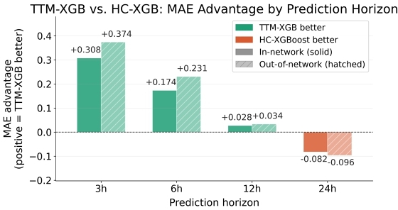
Feature Complementarity Analysis. We compare TTM-XGB (TTM-derived features only) and HC-XGB (44 hand-crafted features only) to isolate each feature type's contribution. As shown in Figure 2, TTM-XGB significantly outperforms HC-XGB at short horizons (3–6h) but underperforms at longer horizons (24h). At short horizons, atmospheric persistence makes TTM's temporal representations more informative than coarse hand-crafted aggregates; at longer horizons, the decisive signals shift to physical prerequisites for frost that domain features directly encode. The full hybrid model outperforms both ablations at every horizon and in both in- and out-of-network settings, confirming the two feature sets are genuinely complementary.
Zero-Shot vs. Trained Temporal Encoder. To demonstrate the benefit of using zero-shot TTM as the temporal encoder, we replace it with (1) a fine-tuned TTM (TTM-FT+XGB) and (2) deep sequence models trained from scratch (GRU+XGB, TCN+XGB), all paired with the same domain features and XGBoost. Table 2 shows that our model consistently achieves the lowest MAE across all horizons on both temporal and spatial hold-outs. All three trained variants underperform our model. Whether fine-tuning a pre-trained encoder or training from scratch, adapting to a geographically limited station dataset introduces station-specific patterns that do not generalize to unseen sites. These results confirm that zero-shot deployment of a pre-trained TSFM achieves superior accuracy and spatial robustness over all trained encoder alternatives.
| Model | 3h | 6h | 12h | 24h | ||||
|---|---|---|---|---|---|---|---|---|
| T | S | T | S | T | S | T | S | |
| TTM-FT+XGB | 1.227 | 1.327 | 1.447 | 1.563 | 1.650 | 1.814 | 1.853 | 2.037 |
| GRU+XGB | 1.263 | 1.424 | 1.389 | 1.562 | 1.492 | 1.679 | 1.624 | 1.831 |
| TCN+XGB | 1.257 | 1.426 | 1.378 | 1.565 | 1.487 | 1.684 | 1.617 | 1.834 |
| Ours | 0.930 | 1.036 | 1.143 | 1.279 | 1.363 | 1.538 | 1.554 | 1.766 |
5 Conclusion
In this study, we proposed a hybrid frost prediction framework combining zero-shot temporal representations with domain-knowledge hand-crafted features. Ablations confirm a horizon-dependent complementarity: temporal representations dominate at short horizons via atmospheric persistence, while hand-crafted features prevail at longer horizons where physical boundary conditions and geographic controls govern frost formation. Our model achieves the highest AUPRC and Brier score at ≥ 6 hours on both temporal and spatial holdouts, with substantially smaller generalization degradation than purely temporal baselines.
Acknowledgments
This research is supported by UC Merced Spring 2023 Climate Action Seed Competition Grant, CAHSI-Google Institutional Research Program Award, and F3 R&D GSR Award funded by the US Department of Commerce, Economic Development Administration Build Back Better Regional Challenge.
References
- Shaojie Bai, J Zico Kolter, and Vladlen Koltun. 2018. An empirical evaluation of generic convolutional and recurrent networks for sequence modeling. arXiv preprint arXiv:1803.01271 (2018).
- Milad Barooni, Koorush Ziarati, and Ali Barooni. [n. d.]. Frost Prediction Using Machine Learning Methods in Fars Province. In 2023 28th International Computer Conference, Computer Society of Iran (CSICC). IEEE, 25–26. https://doi.org/10.1109/CSICC58665.2023.10105391
- Sandeep Bhatti, Peter Jeranyama, Casey D Kennedy, Anthony R Buda, David J Millar, Adrian RH Wiegman, and Juan Zalapa. 2025. Forecasting spring frost events in agriculture using machine learning: A case study from southeastern Massachusetts, United States. Smart Agricultural Technology (2025), 101720.
- Ed Brotak. 2014. The Big Freeze: Frost's Costly Impact on Agriculture. Weatherwise 67, 1 (2014), 30–35.
- Tianqi Chen and Carlos Guestrin. 2016. XGBoost: A Scalable Tree Boosting System. In ACM Conferences. Association for Computing Machinery, New York, NY, USA, 785–794. https://doi.org/10.1145/2939672.2939785
- Kyunghyun Cho, Bart Van Merriënboer, Çağlar Gulçehre, Dzmitry Bahdanau, Fethi Bougares, Holger Schwenk, and Yoshua Bengio. 2014. Learning phrase representations using RNN encoder–decoder for statistical machine translation. In Proceedings of the 2014 conference on empirical methods in natural language processing (EMNLP). 1724–1734.
- Ana Laura Diedrichs, Facundo Bromberg, Diego Dujovne, Keoma Brun-Laguna, and Thomas Watteyne. 2018. Prediction of frost events using machine learning and IoT sensing devices. IEEE Internet of Things Journal 5, 6 (2018), 4589–4597.
- Écio Souza Diniz, Alexandre Simoes Lorenzon, Nero Lemos Martins de Castro, Gustavo Eduardo Marcatti, Osmarino Pires dos Santos, José Carlos de Deus Júnior, Rosane Barbosa Lopes Cavalcante, Elpídio Inácio Fernandes-Filho, and Cibele Hummeldo Amaral. 2021. Forecasting frost risk in forest plantations by the combination of spatial data and machine learning algorithms. Agricultural and Forest Meteorology 306 (2021), 108450.
- Vijay Ekambaram, Arindam Jati, Pankaj Dayama, Sumanta Mukherjee, Nam H Nguyen, Wesley M Gifford, Chandra Reddy, and Jayant Kalagnanam. 2024. Tiny time mixers (ttms): Fast pre-trained models for enhanced zero/few-shot forecasting of multivariate time series. Advances in Neural Information Processing Systems 37 (2024), 74147–74181.
- Hyojeoung Kim, Jong-Min Kim, and Sahm Kim. 2022. Frost Forecasting considering Geographical Characteristics. Adv. Meteorol. 2022, 1 (Jan. 2022), 1127628. https://doi.org/10.1155/2022/1127628
- Taesung Kim, Jinhee Kim, Yunwon Tae, Cheonbok Park, Jang-Ho Choi, and Jaegul Choo. 2021. Reversible instance normalization for accurate time-series forecasting against distribution shift. In International conference on learning representations.
- Yuxuan Liang, Haomin Wen, Yuqi Nie, Yushan Jiang, Ming Jin, Dongjin Song, Shirui Pan, and Qingsong Wen. 2024. Foundation models for time series analysis: A tutorial and survey. In Proceedings of the 30th ACM SIGKDD conference on knowledge discovery and data mining. 6555–6565.
- Tsung-Yi Lin, Priya Goyal, Ross Girshick, Kaiming He, and Piotr Dollár. 2017. Focal loss for dense object detection. In Proceedings of the IEEE international conference on computer vision. 2980–2988.
- Tianhong Liu, Songchao Zhang, Tao Sun, Cong Ma, and Xinyu Xue. 2025. Review of active plant frost protection equipment and technologies: Current status, challenges, and future prospects. Agronomy 15, 5 (2025), 1164.
- Ebrahim Mesgari, Peyman Mahmoudi, Yahya Kord Tamandani, Taghi Tavousi, and Seyed Mahdi Amir Jahanshahi. 2024. A comparative assessment of the ability of different types of machine learning in short-term predictions of nocturnal frosts. Acta Geophysica 72, 4 (2024), 2955–2973.
- K Papagiannaki, K Lagouvardos, V Kotroni, and G Papagiannakis. 2014. Agricultural losses related to frost events: Use of the 850 hPa level temperature as an explanatory variable of the damage cost. Natural Hazards and Earth System Sciences 14, 9 (2014), 2375–2386.
- Javier Pérez Tárraga, Manuel Castillo-Cara, Enrique Arias-Antúnez, and Diego Dujovne. 2025. Frost forecasting through machine learning algorithms. Earth Sci. Inf. 18, 2 (June 2025), 183. https://doi.org/10.1007/s12145-025-01710-6
- José Roberto Rozante, Enver Ramirez, Diego Ramirez, and Gabriela Rozante. 2023. Improved frost forecast using machine learning methods. Artificial Intelligence in Geosciences 4 (2023), 164–181.
- Huan Song, Lijun Wang, Yongguang Hu, Jie Yang, and Jinxing Niu. 2025. Multi-component gradient enhancement for accurate frost detection and quantification on leaf surfaces. Scientific Reports 15, 1 (2025), 34684.
- Carl J Talsma, Kurt C Solander, Maruti K Mudunuru, Brandon Crawford, and Michelle R Powell. 2023. Frost prediction using machine learning and deep neural network models. Frontiers in Artificial Intelligence 5 (2023), 963781.
- Fred Torres-Cruz, Dina Maribel Yana-Yucra, and Richar Andre Vilca-Solorzano. 2025. Comparative Analysis of Statistical, Machine Learning, and Deep Learning Approaches for Frost Prediction in the Peruvian Altiplano.International Journal of Advanced Computer Science & Applications 16, 9 (2025).
Footnote
1 https://rapidrefresh.noaa.gov/hrrr/
2 https://www.ncei.noaa.gov/products/weather-climate-models/numerical-weather-prediction

This work is licensed under a Creative Commons Attribution 4.0 International License.
ACM Sustainability Week Companion '26, Banff, AB, Canada
© 2026 Copyright held by the owner/author(s).
ACM ISBN 979-8-4007-2199-1/26/06.
DOI: https://doi.org/10.1145/3765611.3815487